COMSOL Under Pressure
Sometimes you need to model the concentration of a gas in a liquid or a gas-permeable solid. You can work out simple models by hand using mass transport principles, but more complicated models require finite element software. Unfortunately COMSOL is ignorant of Henry’s law, but you can bring it up to speed through the clever use of boundary conditions.
A Little Background
The idea that a gas exerts pressure is familiar to anyone who has ever over-inflated a balloon. The gas molecules bounce around, hitting each other and the wall of the balloon. A gas can dissolve in liquids and some solids (e.g., polymers) and because the gas molecules are bouncing around they exert pressure on the liquid or solid molecules as well. Even though the gas is dissolved, it still has a pressure.
Mixtures of gasses work the same way. Air is made up of a mixture of gases and each gas contributes its own partial pressure.
where is the partial pressure of oxygen, is the partial pressure of carbon dioxide, and so on. The partial pressure of oxygen in air is about 160 mmHg.
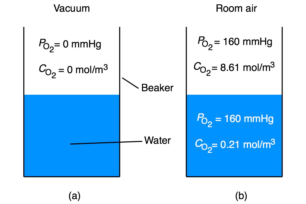
Imagine that a beaker half full of water has been sitting in a vacuum chamber overnight so that no gas is dissolved in the water (Figure 1a). You take the beaker out and let it sit in air at normal temperature (20 °C) and pressure (760 mmHg) until it equilibrates, as shown in Figure 1b. Once the system reaches equilibrium, the partial pressure of oxygen will be the same in the air and the water, but the concentration will be different. The water molecules take up space, so there cannot be as many oxygen molecules per unit volume in the water even though the partial pressures are equal. At normal temperature and pressure (20 °C and 760 mmHg) the concentration of oxygen in air is 8.61 mol/m and in water at is 0.21 mol/m.
Henry’s law is used to relate the concentration of a gas to its partial pressure. The affinity that a gas molecule has for a liquid or solid phase is called its solubility coefficient, or . Henry’s law is
where is the partial pressure of gas , is the concentration of gas , and is solubility coefficient of dissolved gas . Some common solubility coefficients are listed below.1
| Gas | |
|---|---|
| O | 0.024 |
| CO | 0.570 |
| CO | 0.018 |
| N | 0.012 |
| He | 0.008 |
Why Use Henry’s Law in COMSOL?
Unfortunately COMSOL is unaware of the concept of solubility. If you model the beaker in Figure 1 in COMSOL using steady-state analysis you will get the results shown in Figure 2.
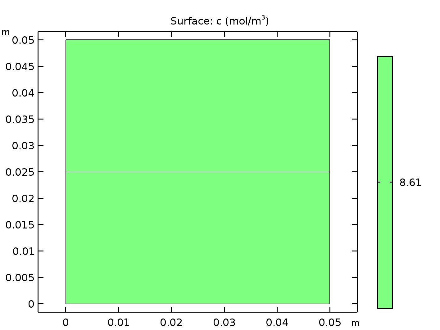
These results look good except for the fact that COMSOL is lying. COMSOL is telling us that there are 8.61 mol/m of oxygen in the air above the beaker and in the water in the beaker. If you read the section above on Henry’s law, then you know that this is codswallop. It is true that the partial pressures of oxygen are the same in the air and the water, but not the concentrations. Instead, we have to use Henry’s law to figure out what the concentration is in the water. In this case the pressure of oxygen in the air, , is equal to the pressure of oxygen in the water, , or
Using Henry’s law we have
where is the concentration of oxygen in the air, is the concentration of oxygen in water and is the solubility of oxygen in water. The constant does not really exist because solubilities are measured with respect to the gas phase, so we can assign it a value of one. We can find the concentration of oxygen in water with
In other words, all we have to do to find the concentration of oxygen in water is scale the solution that COMSOL finds by the consant . If we multiply 8.61 mol/m by 0.024 then we get an oxygen concentration in water of 0.21 mol/m. You could take this approach in all your COMSOL simulations, however a much better way is to make COMSOL do it for you.
How to Use Henry’s Law in COMSOL
You can get COMSOL to implement Henry’s Law via boundary conditions. The trick is to (1) assign a physics to each material in your model and (2) assign a flux boundary condition at each interface between materials. In the beaker model above, there are two materials (water and air) and one interface between them. Since we have two domains in the COMSOl model we need to assign the flux boundary condition in each domain. The formula for inward flux at the boundary follows this form:
Here is the gas concentration in the neighboring domain, is the gas concentration in the reference (i.e., current) domain, is the gas solubility in the current domain, and is the gas solubility in the adjacent domain. You can generate the two boundary conditions for the beaker model using this pattern. In the air domain the boundary condition at the air/water interface is
and in the water domain the boundary condition at the air/water interface is
The variable is the stiff spring velocity and should be a fairly large value. I used 100000 m/s. (Update: a large value may not always work—see note below2)
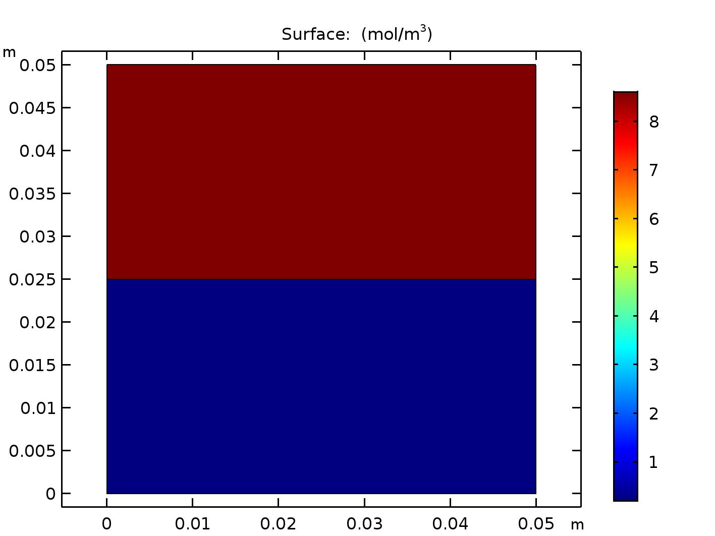
Now when you run COMSOL you get the result shown in Figure 3. Each domain has a uniform concentration of O, but the concentrations in each domain are different, as expected (8.61 mol/m in the air domain and 0.21 mol/m in the water domain).
This approach to modeling solubilities in COMSOL can be extended to models with many different domains. Just be sure that you follow the correct pattern when assigning your flux boundary conditions.
A Quick Note on Plotting Your Results
You will need to assign a physics to each domain (material) in your model if you want to account for solubility in COMSOL. The water beaker model shown above consisted of two domains, each assigned the transport of dilute species (tds) physics. By default, COMSOL will produce two output plots for this model: one for the air domain and one for the water domain, shown below.
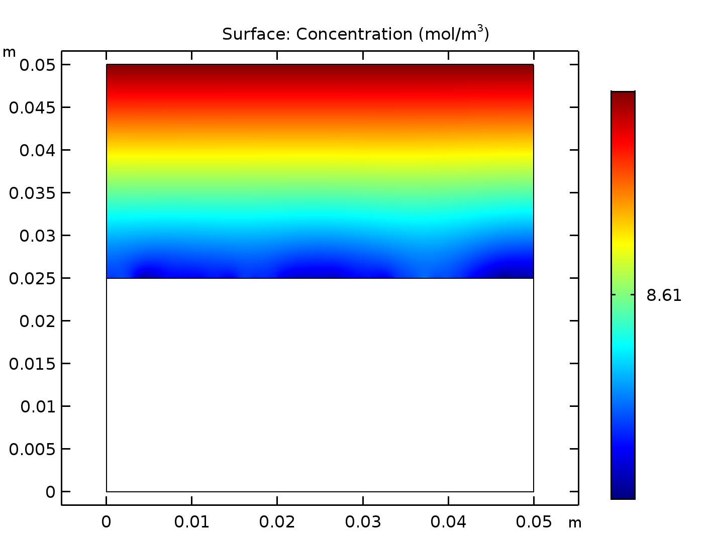
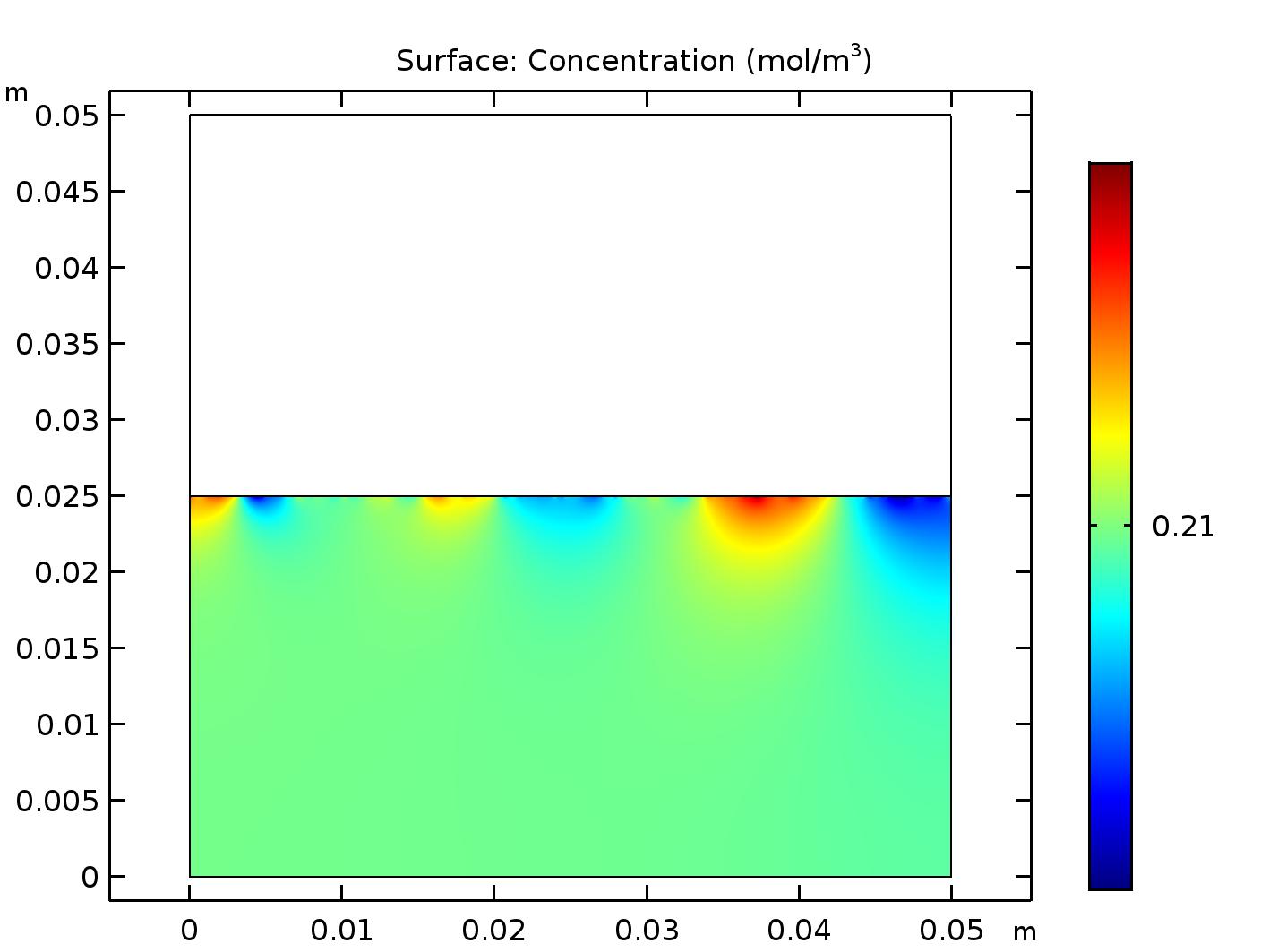
There are a variety of colors in these surface plots, but they are due to rounding errors and in fact represent the same concentration of oxygen in each domain. Incorporate both of these results into a single plot by following these steps:
- Under
Component -> Definitionadd two variables. In one of the variables enter aNamethat will represent your composite plot. I used . Under theExpressioncolumn enter one of your concentration variables. I used for water concentration inVariable 1. I did the same forVariable 2, but used as myExpressionvalue. - Go to
Resultsand add a new2D Plot Group. Under this new group add a newSurfaceplot. - In the new surface plot settings go to the
Expressionheading and enter the variable name for your composite plot. In my case I entered . Run the plot and you will have an output like that shown in Figure 3.
Supplementary Information
- Link to COMSOL file for simulation without solubility.
- Link to COMSOL file for simulation with solubility.
Guyton, A. and Hall, J. (1996), Textbook of Medical Physiology. Philadelphia: Saunders.↩︎
Update from August, 2018: Dunzhu Li from Trinity College Dublin writes that a very small value, such as 1e-5 m/s, worked for his 2D and 3D models. So if your model does not converge with a large spring constant, try a very small value.↩︎