Lesson 10

1 Learning Objectives

By the end of this lesson students will be able to:

• Write the DE of a second order system
• Determine the roots of a second order system
• Classify the output of a second order system as undamped, underdamped, critically damped, or overdamped
• Write the equation form of the step response of a second order system
• Calculate the damped frequency of an underdamped second-order system
• Calculate $\zeta$, $\omega_{n}$, $\omega_{d}$, $T_{r}$, $T_{p}$, %OS, and $T_{s}$ of a system
• Determine values for components of a system required to meet design specifications

2 Review

A second-order transfer function can be written two ways.

Form 1:

$$\frac{y(s)}{F(s)} = \left\lbrack \frac{y_{ss}}{\left( \frac{1}{{\omega_{n}}^{2}} \right)s^{2} + \left( \frac{2\zeta}{\omega_{n}} \right)s + 1} \right\rbrack$$

Form 2:

$$\frac{y(s)}{F(s)} = \left\lbrack \frac{y_{ss}{\omega_{n}}^{2}}{s^{2} + 2\zeta\omega_{n}s + {\omega_{n}}^{2}} \right\rbrack$$

If the transfer function is in Form 1, the coefficient of $s^{2}$ is equal to $\frac{1}{{\omega_{n}}^{2}}$ and the coefficient of $s$ is equal to $\frac{2\zeta}{\omega_{n}}$.

If the transfer function is in Form 2, the coefficient of $s$ is equal to $2\zeta\omega_{n}$ and the constant is equal to ${\omega_{n}}^{2}$.

Put the transfer function into whichever form makes more sense to you, and then you can solve for $\zeta$ and $\omega_{n}$ by using the coefficients and constant in the denominator polynomial.

3 Overview

Second order systems can have four different types of outputs to a step input:

1. Undamped
2. Underdamped
3. Critically damped
4. Overdamped

We determine what the response will be by either solving for $\zeta$ or by finding the roots of the polynomial in the denominator and plotting them on the complex plane. The roots of the denominator are called poles in control systems lingo. The roots of the numerator are called zeroes.

3.1 A Quick Refresher on Complex Numbers

Use your method of choice to find the roots of the polynomial $s^2 + 2s + 2$. The roots are $s = -1 \pm j$.

3.2 How to Find Roots

1. Use the roots([a b c]) function in MATLAB
2. Use a version of the quadratic equation (when $\zeta < 1$): $s_{1,2} = -\zeta\omega_n\pm \omega_n\sqrt{\zeta^2-1}$
3. Use the quadratic equation: $s_{1,2} = \frac{-b \pm \sqrt{b^2 - 4ac}}{2a}$

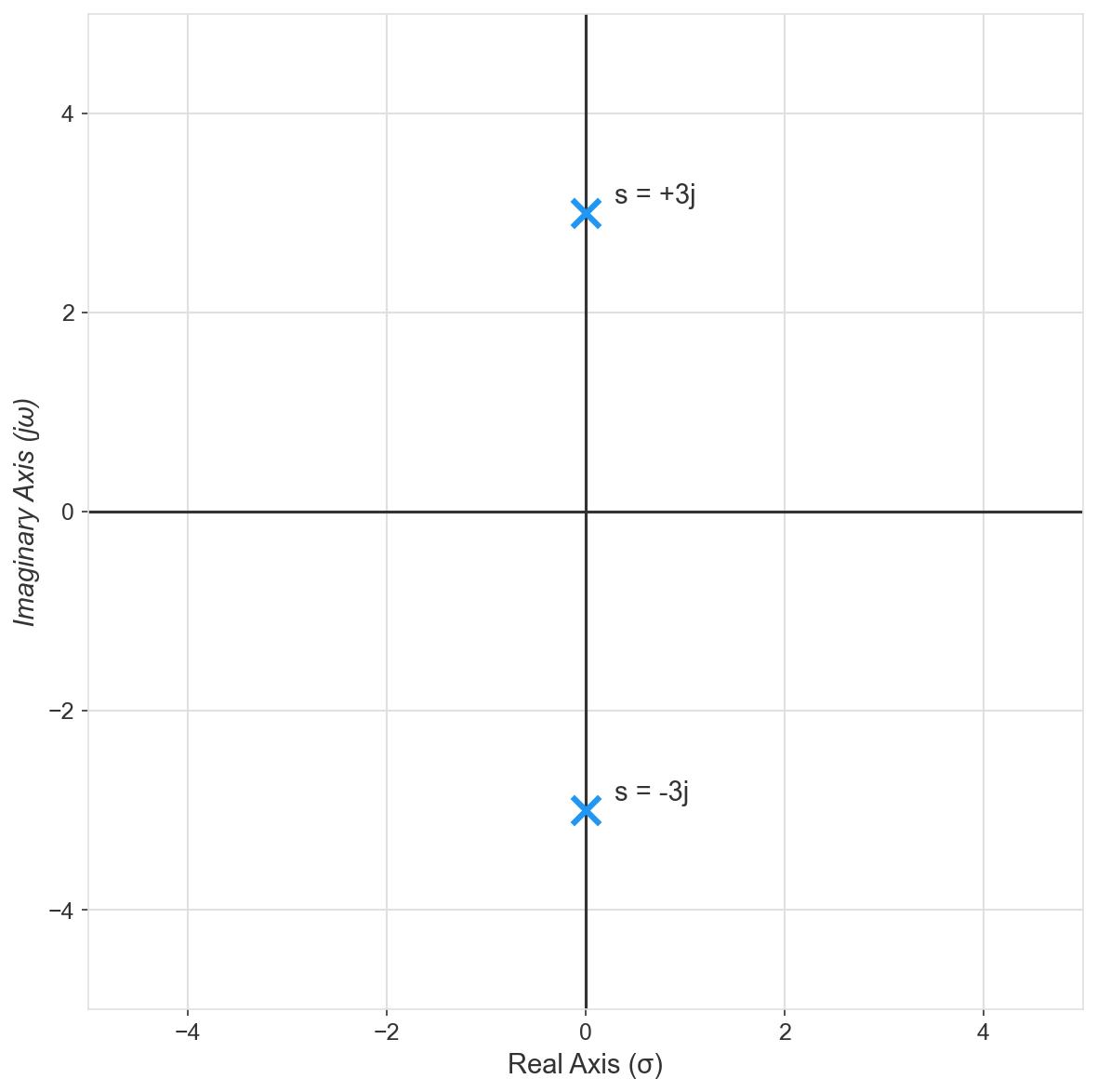
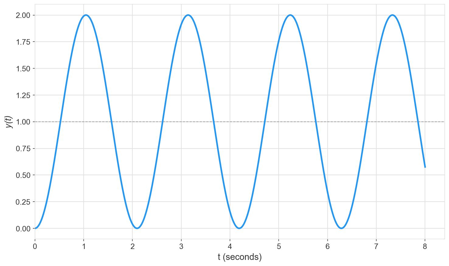
4 Undamped Response ($\zeta = 0$)

When $\zeta = 0$ there is no middle term in the denominator of the polynomial.

Assume the transfer function is

$$G(s) = \frac{1}{\frac{1}{9}s^{2} + 1}$$

Then the roots will be $s_{1,2} = \pm j3$.

And the plot of the poles is:

And the solution of the DE given a step input is:

$$y(t) = 1 - \cos(3t)$$

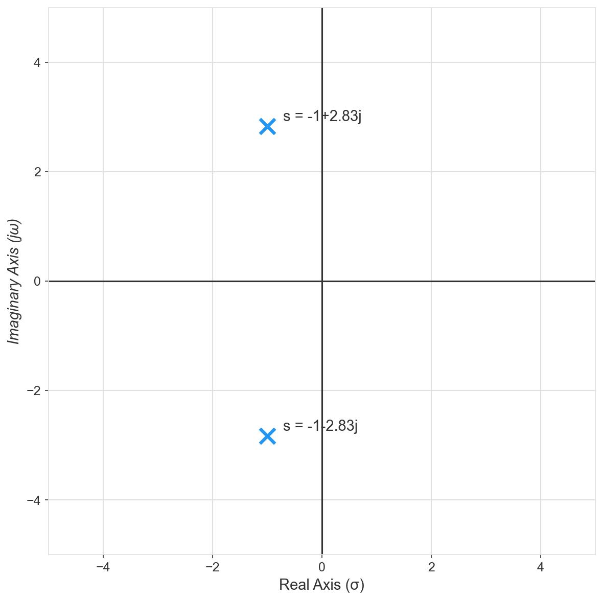
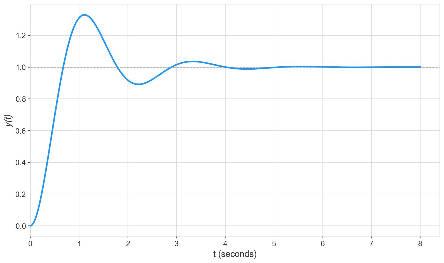
5 Underdamped Response ($0 < \zeta < 1$)

Assume

$$G(s) = \frac{1}{\frac{1}{9}s^{2} + \frac{2}{9}s + 1}$$

Then the roots of the denominator are

$$s_{1,2} = - 1 \pm j2\sqrt{2}$$

The plot of the poles looks like:

And the solution of the DE given a step input is:

$$y(t) = 1 - e^{- t}\left( \cos\left( 2\sqrt{2}t \right) + \frac{\sqrt{2}}{4}\sin\left( 2\sqrt{2}t \right) \right)$$

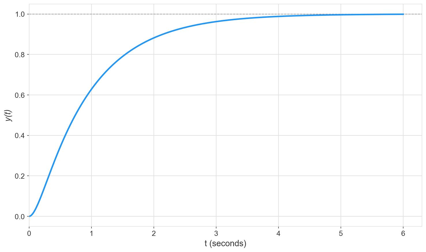
6 Critically Damped Response ($\zeta = 1$)

Assume

$$G(s) = \frac{1}{\frac{1}{9}s^{2} + \frac{6}{9}s + 1}$$

Then the roots of the denominator are

$$s_{1,2} = - 3, - 3$$

The plot of the poles looks like:

And the solution of the DE given a step input is:

$$y(t) = 1 - 3te^{- 3t} - e^{- 3t}$$

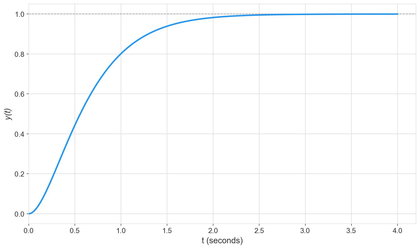
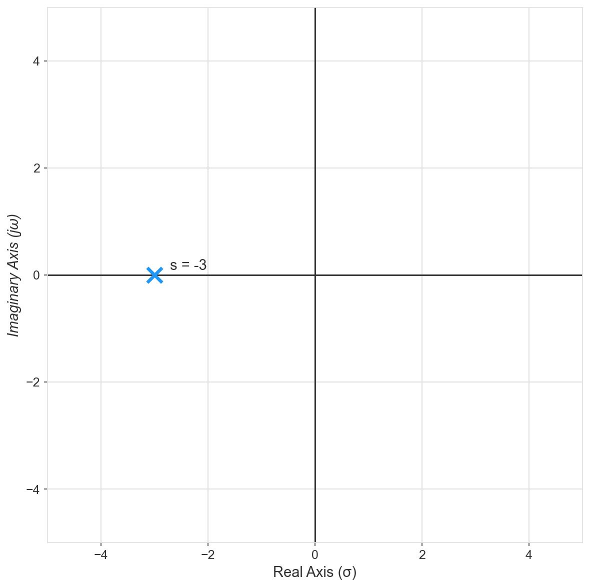
7 Overdamped Response ($\zeta > 1$)

Assume

$$G(s) = \frac{1}{\frac{1}{9}s^{2} + s + 1}$$

Then the roots of the denominator are

$$s_{1,2} = - 7.8541, - 1.1459$$

The plot of the poles looks like:

And the solution of the DE given a step input is:

$$y(t) = 1 + 0.171e^{- 7.854t} - 1.171e^{- 1.146t}$$

8 Comparison of All Four Responses

8.1 Student Exercise 1

Given: Four transfer functions

$$G(s) = \frac{400}{s^{2} + 12s + 400}$$

$$G(s) = \frac{900}{s^{2} + 90s + 900}$$

$$G(s) = \frac{225}{s^{2} + 30s + 225}$$

$$G(s) = \frac{625}{s^{2} + 625}$$

Required: Determine (1) the $\zeta$ and $\omega_{n}$ of each and (2) the type of response (underdamped, undamped, overdamped, critically damped)

Solution

9 Mathematical Pattern of the Four Response Types

The response (output) of a system modeled by a DE comprises two parts: a homogeneous solution and a particular solution. Or, in mathematical terms

$$y(t) = y_H(t) + y_P(t)$$

The homogenenous solution, $y_H(t)$, is also called the:

• natural response
• free response
• transient response

The particular solution, $y_P(t)$, is also called the:

• forced response
• steady-state response

In controls, we refer to the two solutions as the transient response and the steady-state response. The transient response is determined by the physical components of the system and the steady-state response depends on the system input.

In plain English, the transient response is what the system output looks like when it goes from one steady-state to another steady-state. The steady-state value is what value the system settles down to after the transient disappears.

To get the formula for the transient response, we give the system an impulse input. Mathematically, the transient responses for the four pole locations will always follow the patterns below.

9.1 Overdamped

Two real poles at $- \sigma_{1}, - \sigma_{2}$

$$y_H(t) = K_{1}e^{- \sigma_{1}t} + K_{2}e^{- \sigma_{2}t}$$

9.2 Underdamped

Two complex poles at $- \sigma_{d} \pm j\omega_{d}$

$$y_H(t) = Ae^{- \sigma_{d}t}\cos(\omega_{d}t - \phi)$$

9.3 Undamped

Two imaginary poles at $\pm j\omega_{n}$

$$y_H(t) = A\cos(\omega_{n}t - \phi)$$

9.4 Critically Damped

Two real poles at $- \sigma_{1}$

$$y_H(t) = K_{1}e^{- \sigma_{1}t} + K_{2}te^{- \sigma_{1}t}$$

9.5 Student Exercise 2

Write out the expected form of the solution to each of the transfer functions in Exercise 1.

Matlab code to find the roots

10 Characteristics of the Second Order Transfer Function

10.1 Natural Frequency

Represented by $\omega_{n}$. The frequency of the transient output if it is (or if it were) undamped.

10.2 Damped Frequency

Represented by $\omega_{d}$. The frequency of the output in an underdamped system.

$$\omega_{d} = \omega_{n}\sqrt{1 - \zeta^{2}}$$

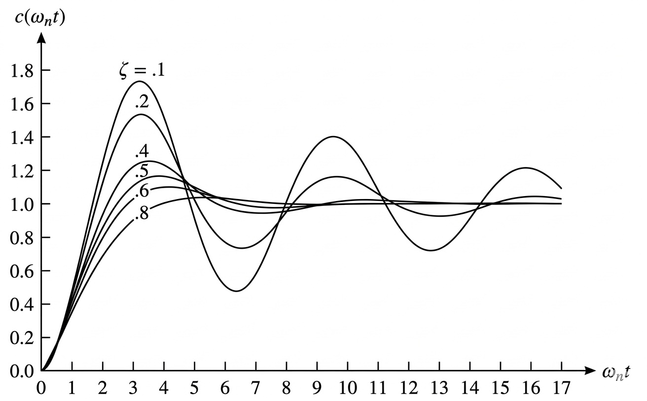
10.3 Damping Ratio

Represented by $\zeta$. How fast an underdamped system dies down to its steady-state.

$$\zeta = \frac{\text{exponential decay frequency}}{\text{natural frequency}}$$

Effect of different $\zeta$ on response:

11 Characteristics of Second Order Systems

Five important features: (1) rise time, $T_{r}$, (2) peak time, $T_{p}$, (3) percent overshoot, %OS, (4) settling time, $T_{s}$.

11.1 Rise Time

Time required for the waveform to go from $0.1y_{ss}$ (10% of steady-state output) to $0.9y_{ss}$ (90% of steady-state output).

No analytical solution is available. Set $y(t) = 0.9$ and $y(t) = 0.1$ and solve for $t$.

11.2 Peak Time

$$T_{p} = \frac{\pi}{\omega_{n}\sqrt{1 - \zeta^{2}}} = \frac{\pi}{\omega_{d}}$$

11.3 Percent Overshoot

$$\%OS = e^{- \left( \zeta\pi/\sqrt{1 - \zeta^{2}} \right)} \times 100$$

Note that you can calculate $\zeta$ if you know %OS:

$$\zeta = \frac{- \ln(\%OS/100)}{\sqrt{\pi^{2} + \ln^{2}(\%OS/100)}}$$

11.4 Settling Time

$$T_{s} = \frac{4}{\zeta\omega_{n}}$$

11.5 Summary Figure

11.6 Exercise 1

Given: The transfer function

$$G(s) = \frac{100}{s^{2} + 15s + 100}$$

Required: $T_{p}$, %OS, $T_{s}$, and $T_{r}$.

wn=sqrt(100)
zeta=15/(2*wn)

tp=pi/(wn*sqrt(1-zeta^2))
os=exp(-zeta*pi/sqrt(1-zeta^2))*100
ts=4/(zeta*wn)

syms s t
y=ilaplace((1/s)*(100/(s^2+15*s+100)))
fplot(y,[0 1])

t1=vpasolve(y==0.1,t,[0 0.2])
t2=vpasolve(y==0.9,t,[0.2 0.4])
t2-t1

11.7 Student Exercise 3

Given: The system shown below.

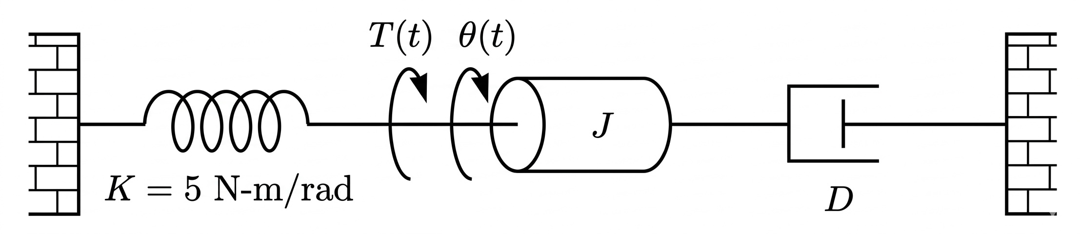
Required: Find $J$ and $D$ to yield 20% OS and a settling time of 2 seconds for a step input to torque.

Solution