Lesson 11

1 Learning Objectives

By the end of this lesson students will be able to:

• Calculate the magnitude and phase of a transfer function given a frequency
• Convert phase angle to time shift and vice versa
• Use magnitude and phase to predict the relative shape of input and output waveforms
• Convert magnitude to dB and vice versa
• Read values from a phase and magnitude plot

2 Introduction

Previously we looked at unit and impulse inputs to systems and plotted their output.

Now we want to see what happens when we use a sine wave as an input.

3 Magnitude and Phase

Consider the following RC circuit:

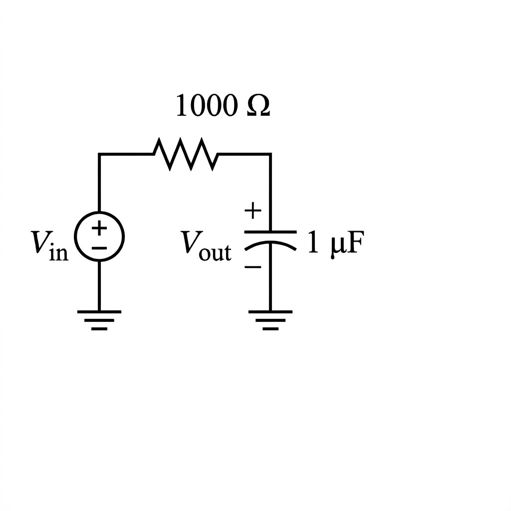
The transfer function is

$$G(s) = \frac{v_{out}}{v_{in}} =$$

Remember that $s = \sigma + j\omega$. But since sinusoidal inputs are steady-state inputs, $\sigma = 0$. So we can re-write $G(s)$ as $G(j\omega)$:

$$G(j\omega) = \frac{v_{out}}{v_{in}} =$$

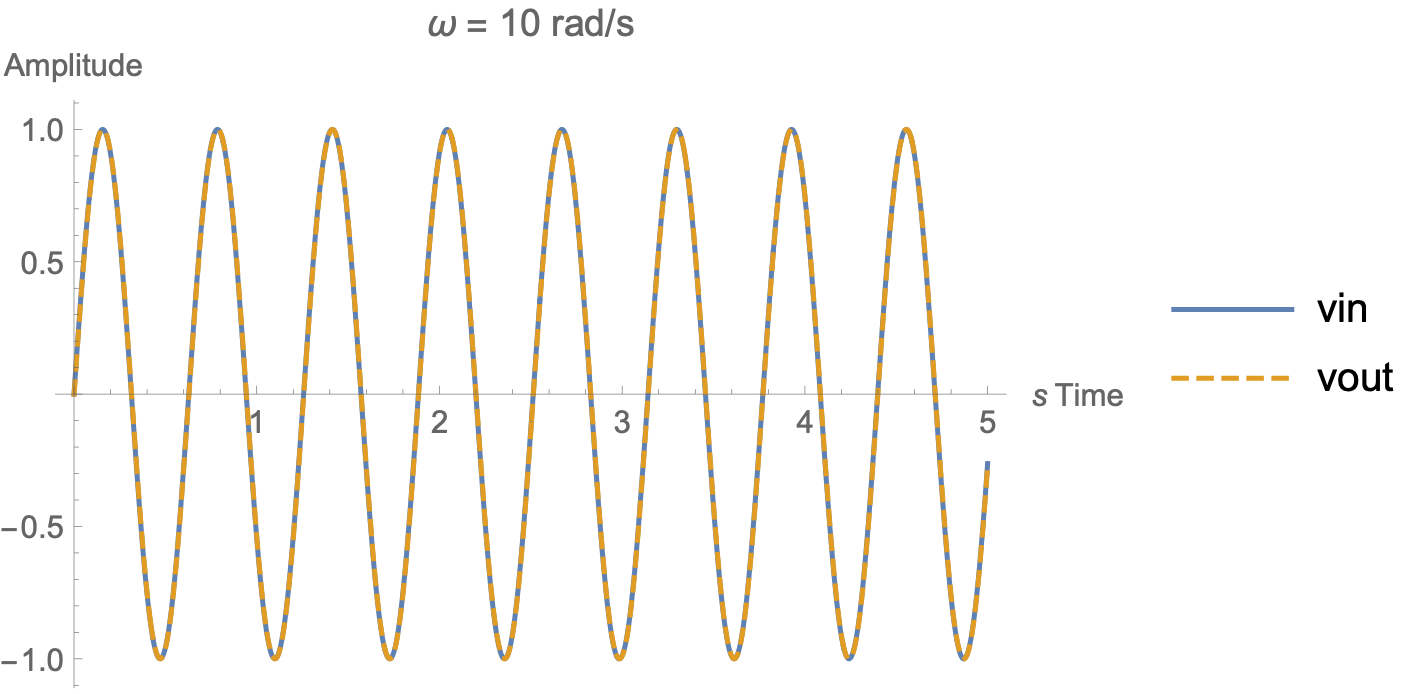
Now, we want to know how the circuit will modify an input sine wave that has a frequency of $\omega = 10$ rad/s. Type in g=1/(0.001*j*10+1) to MATLAB to find out.

$$\frac{v_{out}}{v_{in}} = 1 - j0.01$$

Notice $G(j\omega)$ is now equal to a complex number, which has a magnitude and a phase angle.

In MATLAB, use abs(x) to find the magnitude:

g = 1 - j*0.01
abs(g)

MATLAB will print out 1 which means $|G(j\omega)| = 1$. This is an approximation and the answer is really 1.000049999 if you use vpa(abs(g), 10)

In MATLAB, use angle(x) to find the phase angle:

angle(g)*180/pi

MATLAB will print out -0.5729, which means $\phi = -0.573°$.

3.1 What Do These Numbers Mean?

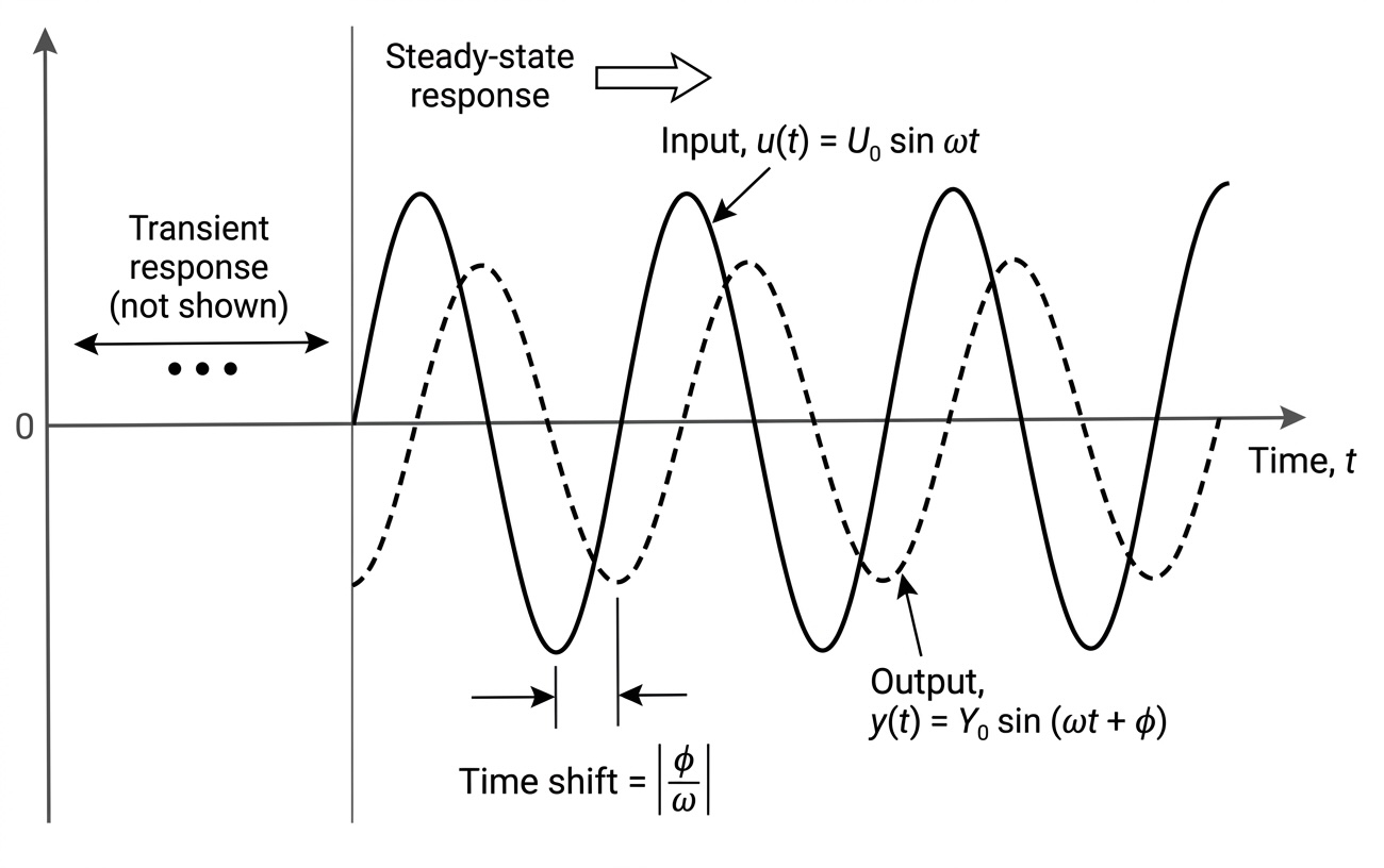
The magnitude of $G(j\omega)$ tells us the ratio of the output amplitude to the input amplitude. The phase angle of $G(j\omega)$ tells us how much the output is shifted in time relative to the input.

Calculate the time shift $\Delta t$ between the two waveforms with

$$\Delta t = \left| \frac{\phi}{\omega} \right|$$

For the previous example:

vpa(abs(angle(g)/10),6)

And MATLAB will output 0.000999967 which means $\Delta t \approx 0.001 \text{ sec} = 1 \text{ msec}$

3.2 Student Exercise 1

Calculate the phase and magnitude of the RC circuit transfer function for frequencies $\omega = 100$, 200, and 500 rad/sec.

Solution

3.3 Student Exercise 2

Use Simulink to simulate the RC circuit above for an input voltage of $2\sin(500t)$ V. Use ode4, fixed time-step of 1e-4, and wire input and output to a single scope. Find sine wave in Source. How does the time shift compare?

Solution

3.4 Student Exercise 3

Determine the formula for the output waveform, $v_{out}(t)$, if the input waveform is $v_{in}(t) = 2\sin(500t)$ V.

4 Phase and Magnitude Plots

We could calculate magnitude and phase for each input, but that would get tedious. It would be much more efficient if we could just see all the phases and magnitudes at once. A computer can quickly calculate each phase and magnitude and plot it—these are called phase and magnitude plots.

Before we get into that, we need to discuss a new type of unit called the decibel.

4.1 Decibels

A decibel is a logarithmic unit written dB (10 dB, 100 dB, -5 dB, and so on).

The formula for converting a magnitude to decibels is

$$G_{dB} = 20\log|G(j\omega)|$$

In this formula, $|G(j\omega)|$ is the magnitude of the transfer function $G(j\omega)$. Use the function abs() in MATLAB to find magnitude. The log function is a base 10 log, so you use log10() in MATLAB.

You have two options for calculating decibels in MATLAB:

1. mag2db(abs(g))
2. 20*log10(abs(g))

4.2 Example 1

Given: $\frac{v_{out}}{v_{in}} = 0.447$

Required: Convert this magnitude to decibels.

$$G_{dB} = 20\log|0.447| = -6.99 \text{ dB}$$

4.3 Student Exercise 4

Convert the following magnitudes to dB.

Solution

4.4 Important Observations about dB

1. If the magnitude of a transfer function is < 1 for a particular $\omega$, it will have a negative dB value.
2. If the magnitude of a transfer function is > 1 for a particular $\omega$, it will have a positive dB value.
3. A magnitude of 1 will give 0 dB. But $\log(1) = 0$, so a value of 0 dB is the same as a magnitude of 1. In other words, in a magnitude plot, a value of 0 dB means you get out what you put in to the system.
4. A factor of 10 difference in magnitude (from 10 to 100, for example) only results in an increase of 20 dB. This fact is important. In other words, every 20 dB the magnitude increases by 10x.

To convert from dB to magnitude use the following formula:

$$|G(j\omega)| = 10^{\frac{G_{dB}}{20}}$$

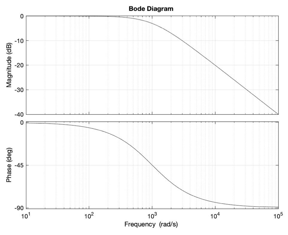
4.5 Bode Plots

Magnitude plots that use dB on the y-axis are often called Bode plots (rhymes with “Okay”). They are semi-log plots because the x-axis is logarithmic while the y-axis is not.

The easiest way to make magnitude and phase plots of a transfer function in MATLAB is to define your transfer function using tf() and then use bode(tf).

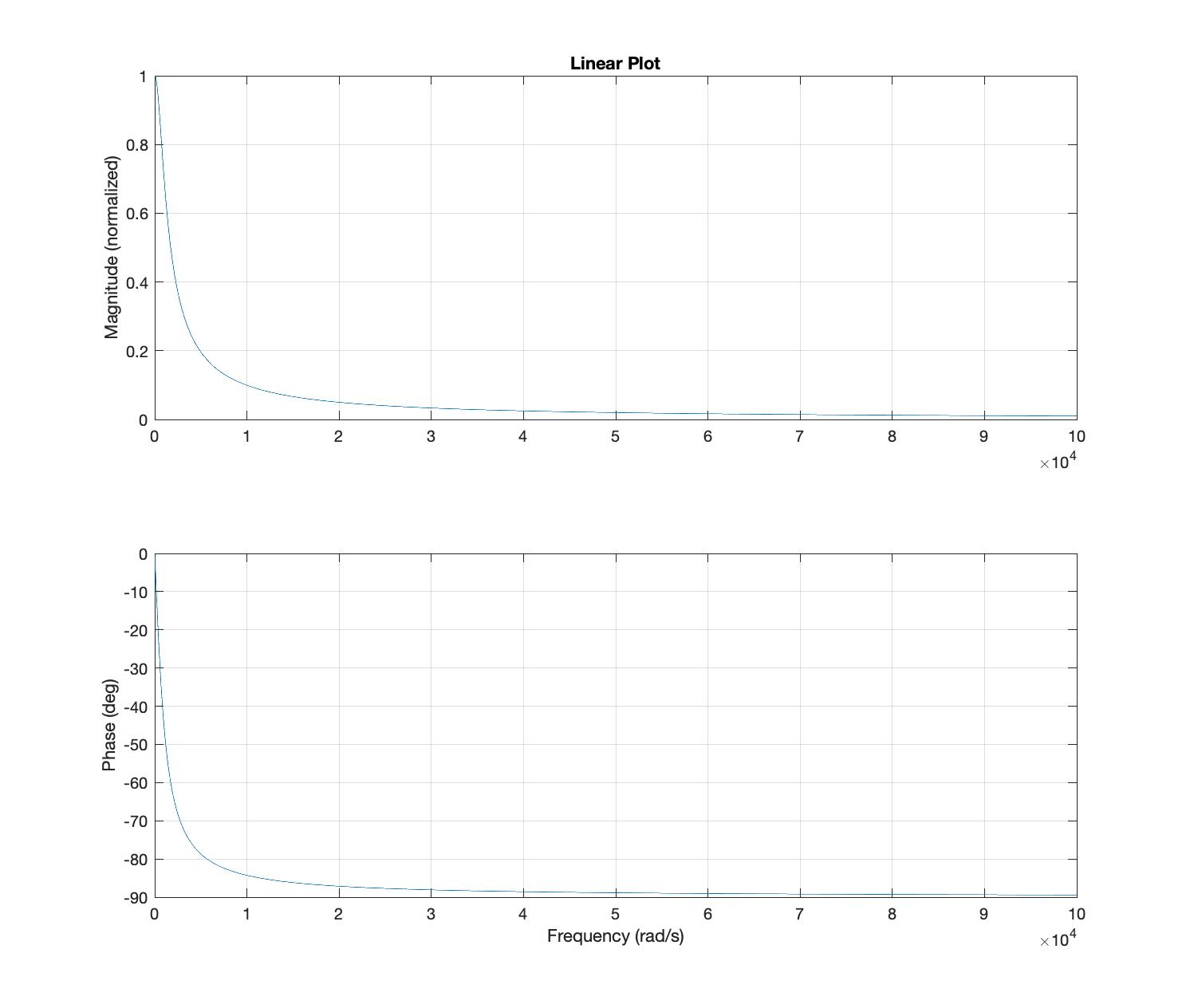
For comparison, here is the same data plotted with a linear (non-logarithmic) x-axis:

4.6 Student Exercise 5

Given: The transfer functions shown below. Generate Bode and phase plots for each.

$$G(s) = \frac{15}{2s + 4}$$

$$G(s) = \frac{3}{s + 7}$$

Required: From the plots for each, estimate $v_{out}(t)$ if $v_{in}(t) = \sin(2t)$ and $v_{in}(t) = 2\sin(15t)$.

Solution