Lesson 12

1 Learning Objectives

By the end of this lesson students will be able to:

• Calculate the cutoff frequency, time constant, and DC gain of a first-order system
• Calculate bandwidth of first and second-order systems
• Explain effect of $\zeta$ on the frequency response of second-order systems
• Design filters with specific cutoff frequencies
• Explain what a filter does
• Calculate the location of the peak in the frequency response of a second-order system

2 What Does the Frequency Response Tell Us?

Previously we looked at unit and impulse inputs to systems and plotted their output. The frequency response of the RC circuit from last time is shown below.

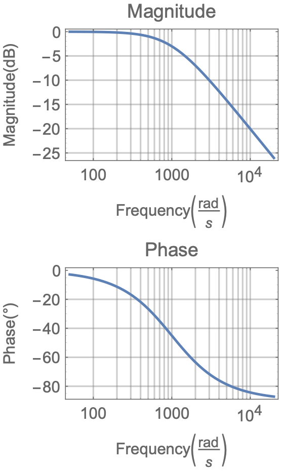
Use Matlab to determine precise values from phase and magnitude plots:

w = 500;
[mag, phase] = bode(G, w)
% mag = 0.8944
% phase = -26.5651

w = 5000;
[mag, phase] = bode(G, w)
% mag = 0.1961
% phase = -78.6901

You can also create phase and magnitude plots with state-space representations after you define the tf.

3 Phase and Magnitude Plots of First-Order Systems

3.1 Standard Form

When we learned about first-order systems this is the equation we used (assuming $y_0 = 0$):

$$y(s) = \frac{y_{ss}}{\tau s + 1}$$

In this equation, $\tau$ is called the time constant and $y_{ss}$ is the steady-state value, but more often $y_{ss}$ is called the DC gain and is represented with a $K$.

$$y(s) = \frac{K}{\tau s + 1}$$

3.2 Effect of DC Gain

Let’s see what effect the DC gain has on the Bode plots.

Assume $G(s) = \frac{K}{0.001s + 1}$

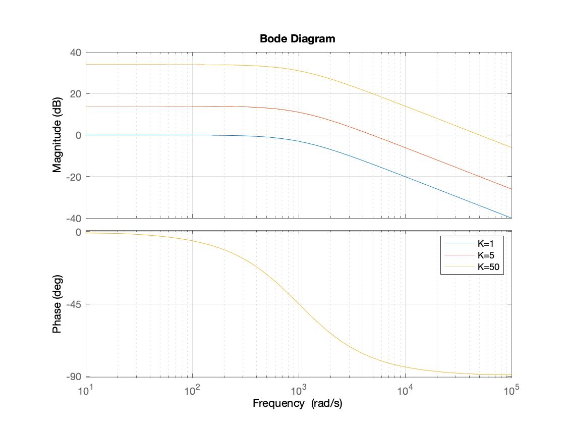
Main points for first-order systems:

1. Increasing $K$ shifts magnitude curve higher
2. Phase plot is not affected by the $K$
3. Phase angle always starts at 0° and approaches -90° at very high frequencies

3.3 Effect of Time Constant

Next, let’s see what effect changing $\tau$ has on the frequency response.

Assume $G(s) = \frac{1}{\tau s + 1}$

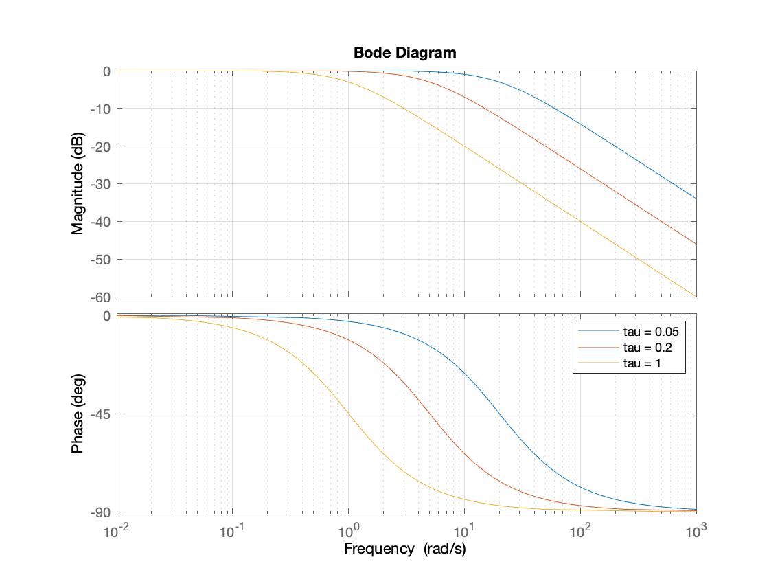
Main points:

1. Phase angle still starts at 0° and ends at -90°
2. $\tau$ changes the frequency of a phase angle of -45°

3.4 Important Points about First-Order Systems

1. The frequency where the phase angle is -45° is known as the cutoff frequency. At this frequency, the magnitude is -3 dB less than the value at 0 rad/sec.
2. The magnitude past the corner frequency is -20 dB/decade.
3. Calculate the cutoff frequency with $\omega_c = 1/\tau$. This is in radians!

3.5 Student Exercise 1

Given: The following transfer function.

$$G(s) = \frac{4}{s + 8}$$

Required: Calculate the DC gain, time constant, and cutoff frequency.

3.6 Student Exercise 2

What DC gain does a first-order system have if the frequency response shows a magnitude of 25 dB for frequencies near 0 rad/sec? Assume a $\tau = 0.001$.

4 Cutoff Frequency

The cutoff frequency is most often used in circuits called filters that remove certain frequencies from a signal and retain others. The cutoff is the threshold.

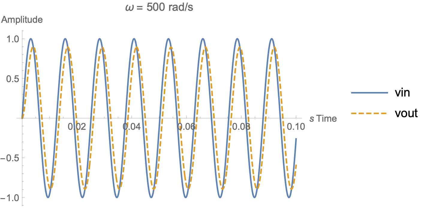
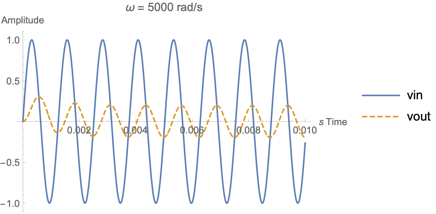
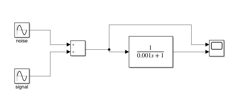
4.1 Example 1

Assume the RC circuit that we have been working with. And that it has a transfer function of $G(s) = \frac{1}{0.001s + 1}$. Assume two inputs: $v_{noise}(t) = 2\sin(2000t)$ and $v_{in}(t) = 2\sin(200t)$.

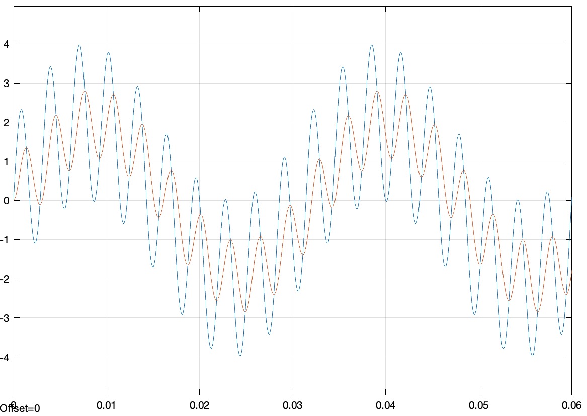
4.2 Student Exercise 3

What amplitudes should $v_{noise}(t)$ and $v_{in}(t)$ have at the output? If you could adjust the frequency for $v_{noise}(t)$, at what frequency would it be 3 dB smaller in amplitude than $v_{in}(t)$?

Solution

5 Phase and Magnitude Plots of Second-Order Systems

Consider the standard form of a second-order system:

$$G(s) = \frac{K\omega_n^2}{s^2 + 2\zeta\omega_n s + \omega_n^2}$$

Assume a second-order system:

$$G(s) = \frac{100}{s^2 + 4s + 100}$$

Key points:

1. Phase angle ranges from 0° to -180°
2. Second-order systems can have a peak in them located at the damped frequency $\omega_r = \omega_n\sqrt{1 - 2\zeta^2}$
3. On magnitude graph, horizontal at low frequencies and then -40 dB/decade over rest

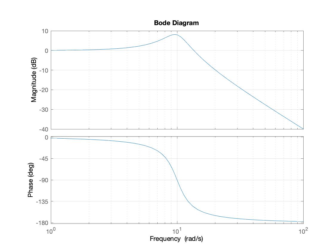
5.1 Effect of $\zeta$ on Bode Plot

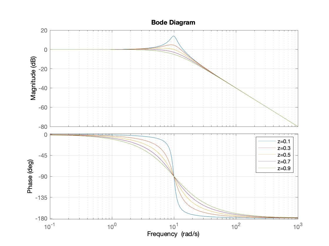
Main points:

1. As $\zeta$ increases, peak magnitude decreases
2. Phase angle transition becomes sharper at lower $\zeta$
3. Phase angle of -90° is the corner frequency $\omega_c$
4. At $\zeta > 0.707$ there is no resonant peak

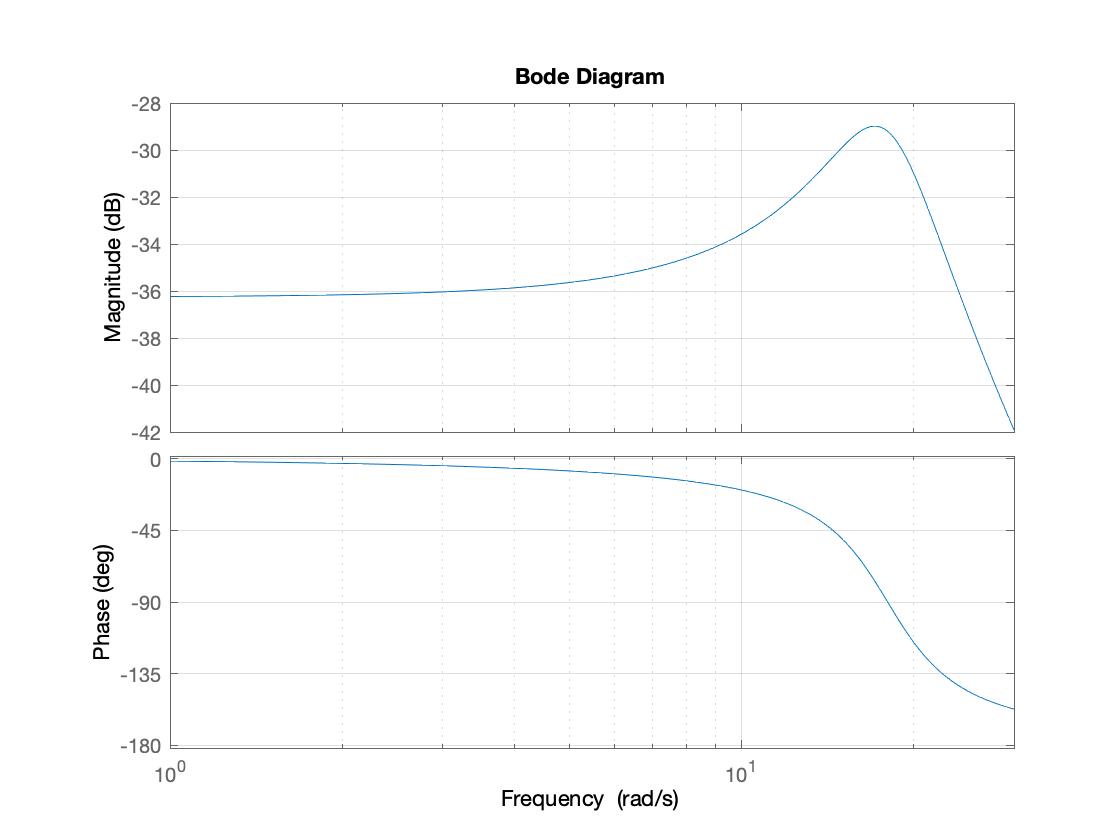
5.2 Student Exercise 4

Given: The transfer function of a rotational system.

$$G(s) = \frac{\theta(s)}{T_{in}(s)} = \frac{1}{0.2s^2 + 1.6s + 65}$$

Required: Generate a Bode plot of the transfer function. Compute the frequency of the peak in the Bode plot. Determine the output if the input is $T_{in}(t) = 1.5\sin(18t)$ N-m.

Solution

6 Bandwidth

The bandwidth is the range of frequencies that a system will stay within 3 dB of the DC gain and up to the cutoff frequency. You can visually determine this from a plot.

6.1 Student Exercise 5

Estimate the bandwidth of the system response plotted below.

You can also use the MATLAB command bandwidth(tf). The answer will be in rad/s.

6.2 Student Exercise 6

Given: The transfer function shown below.

$$G(s) = \frac{5}{s^2 + 8s + 325}$$

Required: Compute the bandwidth of this system.

Solution