Lesson 14
1 Learning Objectives
By the end of this lesson students will be able to:
- Find the equilibrium point of static control systems graphically and with MATLAB
- Implement static control systems in Simulink
2 Introduction
Last time we practiced converting descriptions of physiological systems into control systems. We briefly discussed that the intersection point between the curves will be the equilibrium point. This lesson we practice finding the equilibrium point in systems of varying complexity.
3 Muscle Stretch Reflex
3.1 Exercise 1
Consider the control system for the muscle stretch reflex. This is the knee jerk reflex used in routine medical examinations. The sharp tap to the patellar tendon in the knee stretches the extensor muscle in the thigh. Muscle spindles detect the stretch and transmit a signal along afferent neurons to the spinal cord. The motor neurons in the spinal cord then send a signal along efferent neurons back to the same muscle, in proportion to the afferent firing rate, causing it to contract. In afferent neurons, greater stretch = greater firing rate. In efferent neurons, greater firing rate = more contraction (i.e., shorter muscle length).
3.2 Finding Equilibrium Manually — Linear Equations
If the curves are linear, finding the equilibrium is fairly straightforward. Equations for each block (assume all are linear):
We have three variables: , , . Now the question is what is the equilibrium value of each? We can combine two of the blocks into one like this:
And now that we have only two plots, we can lay them on top of one another:
In summary:
If you have experimental data, you can plot the curves and measure where they intersect. However, you can only get approximate coordinates by doing this (which may be good enough).
Alternatively, if you have more than two curves, it is impractical to use the plotting method and you should instead solve the equations. Using the equations for the two curves from above, we have:
We can use MATLAB to solve for these, especially if there are more than two equations.
3.3 Finding the Equilibrium Point Using MATLAB and Simulink
In the previous example, we assumed linear equations for each block. This almost never happens with real systems. Here is an updated model based on curves fitted to experimental data:
The key thing to see here is that we cannot use the same approach that we used in the previous method because the equations are non-linear. Instead, we now have two choices:
- MATLAB
- Simulink
3.3.1 MATLAB
In MATLAB we can solve a simultaneous system of equations to find the equilibrium for each variable.
3.3.2 Student Exercise 1
Solve the three equations from above for , , and . Then do a quick check that your answer makes sense by plotting both curves on the same graph.
clear all

% Solve equations
syms L fe fa
eqn1 =
eqn2 =
eqn3 =
[L,fe,fa] = vpasolve([eqn1,eqn2,eqn3],[L,fe,fa])

% Plot
clear all;
fe=0:0.01:1;
L= %enter equation for L here
plot(fe,L)
hold on
clear fe;
L=0:0.1:1;
fe= % enter equation for fe here
plot(fe,L)
xlabel("fe");
ylabel("L")
legend(["muscle","spindle"])Using MATLAB to solve simultaneous equations works in many instances, but it will not work with discontinuous functions, which are common in physiological systems. Instead, you must use Simulink.
3.3.3 Simulink
- Use a MATLAB Function (fcn) block for each equation
- Use IC to specify an initial condition to get the loop started
- Run the simulation
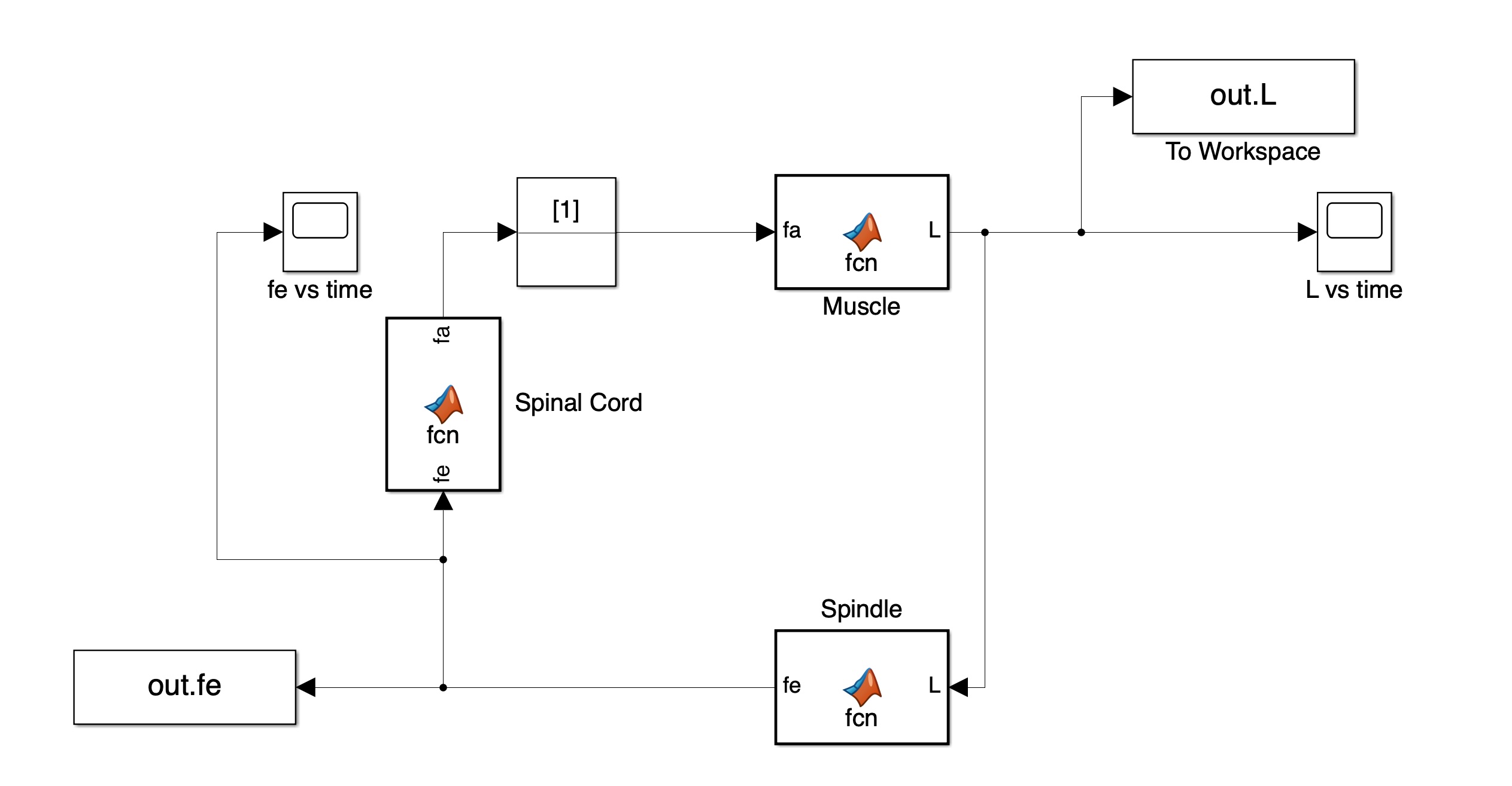
3.3.4 Student Exercise 2
Build the muscle stretch reflex model in Simulink. Use MATLAB Fcn blocks for the muscle, spindle, and spinal cord. Use an Initial Condition block (IC) with a value of 1 and put it in the loop. Use Scope blocks to visualize the output of the muscle block and spindle block. Use To Workspace blocks to send numerical values to MATLAB. Use the ode15s variable step solver and run for 10 sec.
4 Modeling the Regulation of Ventilation
Now we consider how to make a simple model of the chemoreflex regulation of respiration. The important feature of this model is that it contains non-linear piecewise equations (i.e., saturation) that cannot be modeled by simultaneously solving the equations; a numerical approach such as Simulink is the only way.
Breathing rate is controlled mainly by , the concentration of CO in arterial blood. As CO rises, ventilation rate increases, and vice versa. At the same time, a decrease in levels (e.g., from climbing a mountain) will also increase ventilation rate. The increased ventilation rate will increase O levels and decrease CO levels, which in turn lowers ventilation rate. For the purposes of this example, consider two systems: the respiratory controller and the lungs.
Diagram of the system:
The equations for this system are:
The definitions of each variable:
| Variable | Description |
|---|---|
| CO concentration in arterial blood | |
| CO concentration in air (inspired) | |
| Metabolic production rate of CO | |
| Ventilator controller output | |
| O concentration in arterial blood | |
| O concentration in air (inspired) | |
| Metabolic production rate of O |
4.1 Student Exercise 3
Write the code for the three function blocks. Add two constants: one for mmHg (21% O2) and the other for mmHg. Sink all three variable outputs to workspace. Add an IC block for and set it to 2. Run the Simulink model and determine the equilibrium values for , , and .
