Lesson 2

1 Learning Objectives

By the end of this lesson students will be able to:

• Convert a differential equation into LaPlace notation, and vice versa
• List the four standard types of inputs to systems
• Classify differential equations
• Create transfer functions of electrical circuits

2 Mathematical Models of Systems

2.1 How to classify a differential equation

Here is an abstracted version of a differential equation:

$$a_n \frac{d^n y}{dt^n} + a_{n-1} \frac{d^{n-1} y}{dt^{n-1}} + \cdots + a_1 \frac{dy}{dt} + a_0 y = F(t)$$

where:

• $F(t)$ = system input (or forcing function)
• $y(t)$ = system output (or response)
• $t$ = time
• $a$’s = constants

A mathematician calls this equation a linear, ordinary, non-homogeneous differential equation of nth order with constant coefficients.

2.2 Definition of each term

• Linear: none of the terms involve powers or products of $y$ or $dy/dt$. For example, $y^3$ or $(dy/dt)^5$ or $y(dy/dt)$.
• Ordinary: $t$ is the only independent variable. We will be modeling lumped systems in this class. In transport you modeled systems in which position ($x$, $y$, and/or $z$ coordinates) were important. Those are called distributed systems.
• Non-homogeneous: One term on the right hand side that does not contain $y$ or its derivatives. If the equation $= 0$ on the right, then it is homogeneous.
• Differential equation: The equation contains a derivative
• nth order: The $n$ in the highest order derivative determines the differential equation order.
• Constant coefficients: The coefficients, labeled $a$, do not vary with time.

3 Types of Input Signals

There are four: impulse, step, ramp and sinusoid

3.1 Unit Impulse

Also called a Dirac delta function. The mathematical definition is a pulse of magnitude $1/a$ as $a \to 0$. The unit impulse is used to model brief impulses to a system, like a racket hitting a tennis ball.

$$\delta(t) = \lim_{a \to 0} \frac{1}{a} \text{ for } 0 \leq t \leq a$$

3.2 Unit Step

Also called the Heaviside unit function. The function has a value of 0 for $t < 0$ and 1 for $t \geq 0$. The unit step is used to model a sudden shift to a new steady state input. An example might be powering up a circuit, or the wheel of a car hitting a curb and then rolling down a sidewalk.

$$u(t) = \begin{cases} 0 & t < 0 \\ 1 & t \geq 0 \end{cases}$$

3.3 Unit Ramp

This input is used to model moving objects. If we want to create a model of the human eye following an object, we might use the ramp function to model for the motion of the object.

$$r(t) = t u(t) = \begin{cases} 0 & t < 0 \\ t & t \geq 0 \end{cases}$$

3.4 Unit Sinusoid

The unit sinusoid is a waveform that has a frequency. It is used to model sinusoidal phenomena, like breathing or heart rate.

$$x(t) = \sin(\omega t) u(t)$$

4 Writing DEs for Electrical Systems

Electrical systems comprise resistors, capacitors, and inductors. We want to calculate voltage or current. You could write the differential equations for the system, but it’s easier to LaPlace transform the components and then analyze.

Here are the steps:

1. Write $Ls$ for inductor, $\frac{1}{Cs}$ for capacitor, and $R$ for resistor.
2. Solve using Ohm’s law, KCL, KVL, loop, or nodal analysis.

4.1 Example 1

Given the circuit below, find the transfer function $G(s) = \frac{V_C(s)}{V(s)}$.

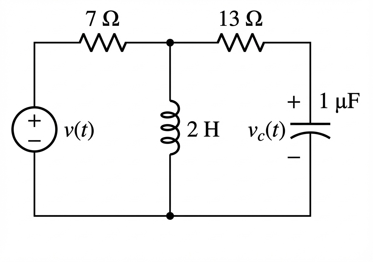
Use MATLAB to solve. Hover over the upper-right corner of the code block to download a Live Script file.

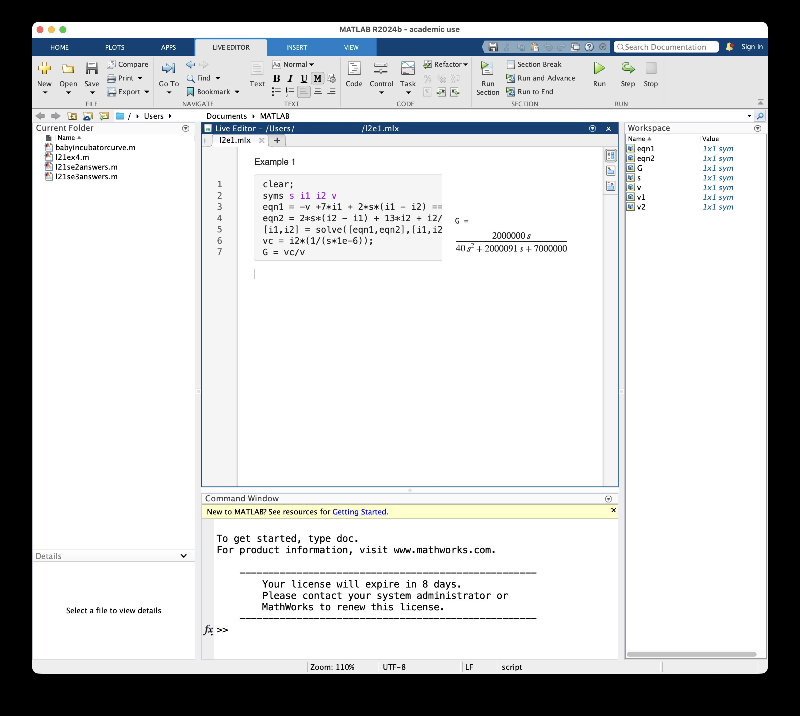
syms s i1 i2 v
eqn1 = -v +7*i1 + 2*s*(i1 - i2) == 0;
eqn2 = 2*s*(i2 - i1) + 13*i2 + i2/(s*1e-6) == 0;
[i1,i2] = solve([eqn1,eqn2],[i1,i2]);
vc = i2*(1/(s*1e-6));
G = vc/v

Result:

$$G(s) = \frac{2000000s}{40s^2 + 2000091s + 7000000}$$

4.2 Student Example 1

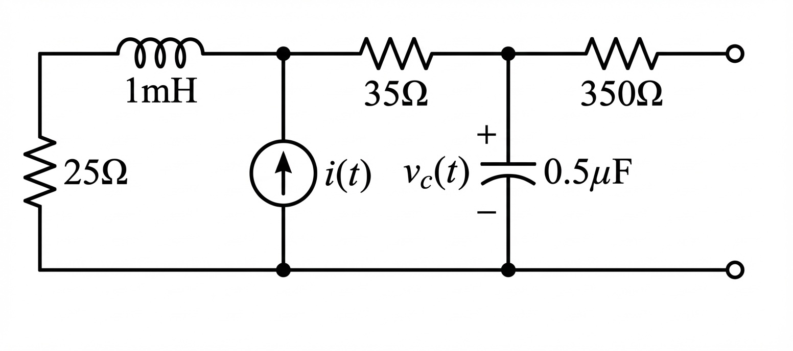
Given the circuit below, find the transfer function $G(s) = \frac{I_B(s)}{I(s)}$. Use MATLAB to solve.

Solution

4.3 Example 2

Given the circuit below, find the transfer function $G(s) = \frac{V_R(s)}{V(s)}$.

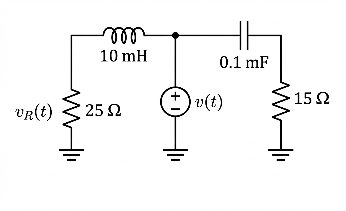
Use MATLAB to solve:

syms s v v1 v2
eqn1 = v1/25 + (v1 - v)/(0.01*s) == 0;
eqn2 = (v2 - v)/(1/(0.1*10^-3*s)) + v2/15 == 0;
[v1,v2] = solve([eqn1,eqn2],[v1,v2]);
G=v1/v

4.4 Student Example 2

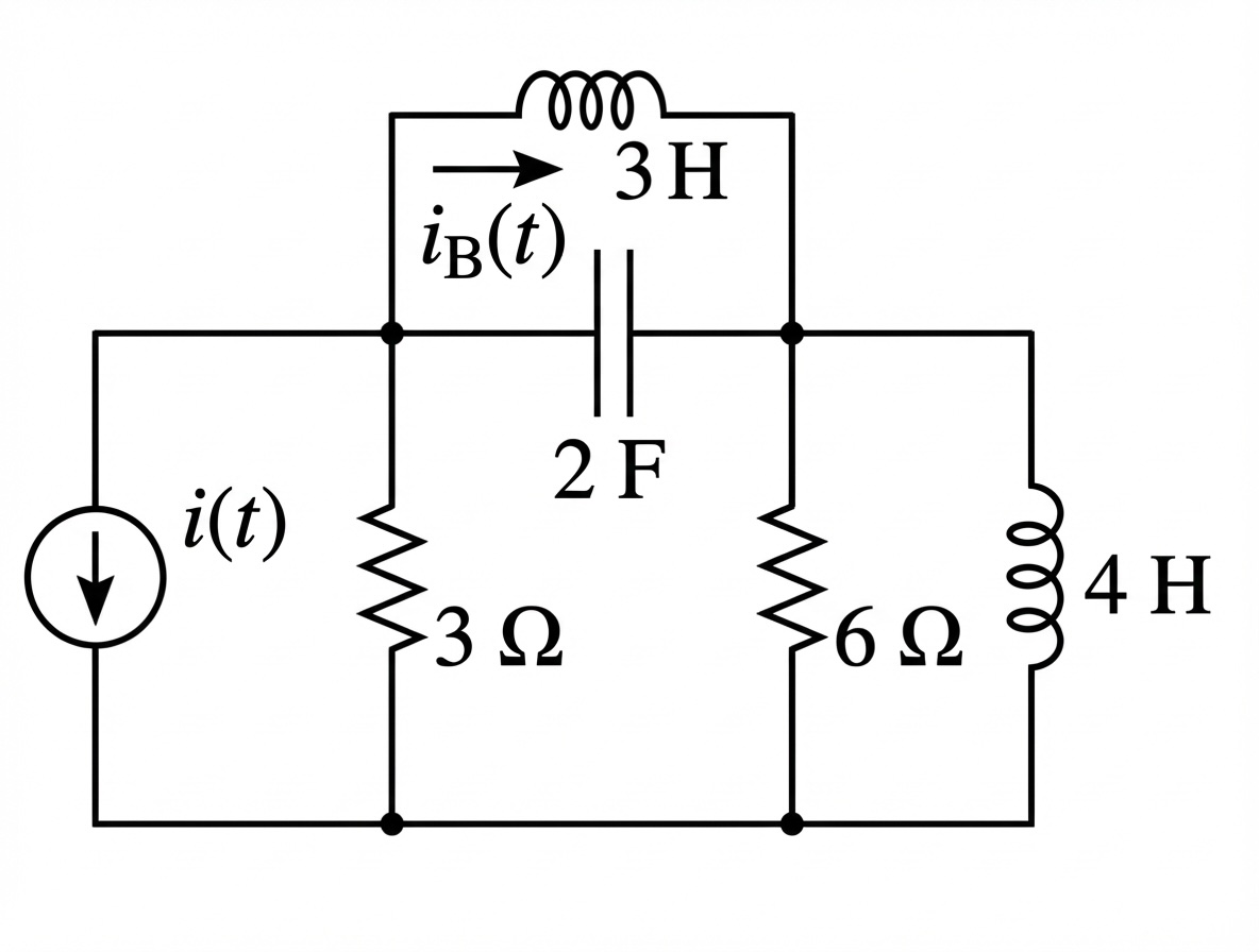
Given the circuit below, find the transfer function $G(s) = \frac{V_L(s)}{V(s)}$. Use MATLAB to solve.

Solution

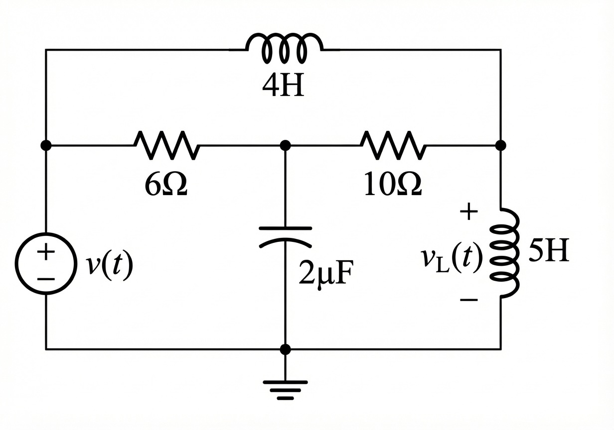
4.5 Student Example 3

Given the circuit below, find the transfer function $G(s) = \frac{V_C(s)}{I(s)}$. Use MATLAB to solve.

Solution