Lesson 17
1 Learning Objectives
By the end of this lesson students will be able to:
- Calculate and for second-order systems with feedback and disturbances if the controller is PID
- Calculate the steady-state output of a system given a step input and PID controller
- Describe the effect a PID controller has on the system response
- Calculate steady-state error for a system with or without a disturbance for any input
- Determine system type and use this information to infer characteristics of the system
- Calculate the error constant of a system
2 Proportional + Integral + Derivative (PID) Controller
Now we add an integral controller to the system:

Now the controller has the transfer function
Plugging this value into our original equation for the ventilator gives
This is a third-order system and there is not a simple analytical formula to calculate the damping ratio or natural frequency. We can make two observations about the system:
- The natural frequency now depends on instead of .
- There is no steady state error because of the integral. Cancel all terms containing and you get .
3 Quick Review of Controllers
To sum up, as briefly as possible, the last lesson-and-a-half:
As engineers, we are given a system:

- We cannot change the plant, , but we want the output to have certain values or characteristics.
- We can build a controller, , that changes the overall transfer function of the system, , and therefore its behavior.
We covered three types of controllers:
- Proportional
- Proportional + Derivative
- Proportional + Integral + Derivative (best)
Each has its pros and cons, but 99% of the controllers you encounter will be PID.
4 Steady-State Errors
With the lung model, we guessed what the steady-state values would be for different systems. The shortcut was to set all and then find the answer from the transfer function. This trick only works for step inputs. Now we practice using a method that always gives the steady-state error, regardless of the type of input.
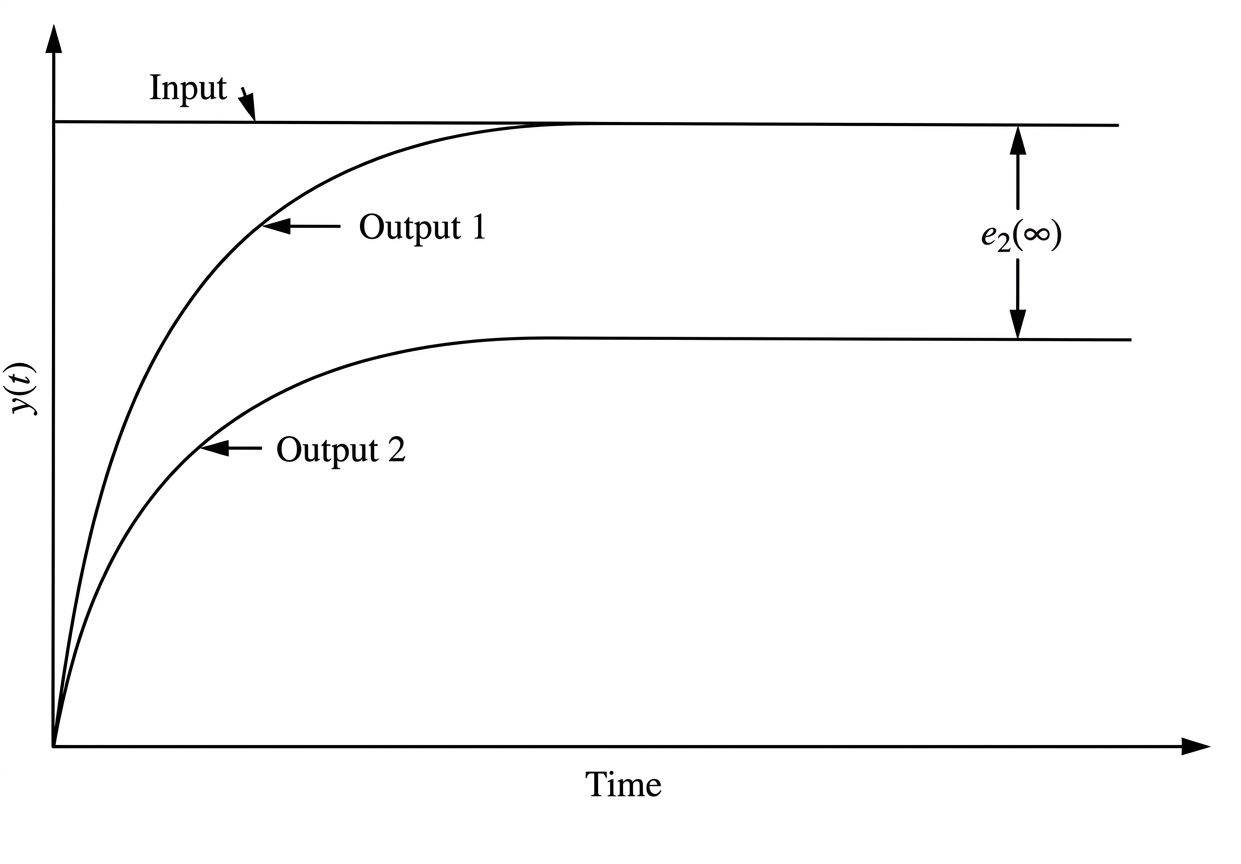
The whole point of a control system is that the output should be equal to what the user chooses as input. The steady-state error of a system is the difference between the system input and output after a very long time, or in math lingo, as .
The method shown below will work for any input, but we limit ourselves to three different types of inputs:
- Step
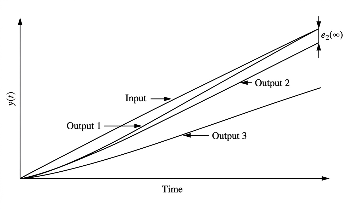
- Ramp
- Parabola
- A system must be stable for you to calculate its steady-state error. You must check the system for stability before calculating the steady-state error. (More on stability in Lesson 18.)
Steady-state error always means the difference between system input and output, but the graph of steady-state error depends on the type of input, as illustrated below.
- You calculate the steady-state error differently for systems with a disturbance and systems without a disturbance.
4.1 Before You Can Calculate Steady-State Error
If the system does not have a disturbance, it must be closed-loop with unity feedback. If it is not, you must convert it to unity feedback before proceeding.
4.2 Steady-State Error for Systems Without a Disturbance
If your unity-feedback system has already been simplified into a single block then use this formula
Otherwise, use this formula
4.2.1 Example 1
Given a unity feedback system with , find the SSE for inputs of , , and .
4.2.2 Student Exercise 1
Given a unity feedback system with , find the SSE for inputs of , , and .
4.3 System Type and Static Error Constants
The free in the denominator of determines system type:
- is Type 0
- is Type 1
- is Type 2
Notice that in the previous example the error values fell into three categories:
- 0
- some number
Static error constants depend on the system type and the type of input:
Step:
Ramp:
Parabola:
In these equations we assume unit inputs (i.e., they have an amplitude of 1). If the inputs are not unit, the amplitude of the input goes in the numerator of each (see Example 1 and Student Exercise 1).
If you know the system type, then you can predict what the steady-state errors will be:
| System Type, N | Unit step input | Unit ramp input | Unit parabola input |
|---|---|---|---|
| 0 | |||
| 1 | 0 | ||
| 2 | 0 | 0 |
4.3.1 Student Exercise 2
Consider a closed-loop system with no disturbance and unity feedback. Assume a proportional controller with gain . The plant transfer function is shown below. What are the steady-state errors of the system to a step, ramp, and parabola input with magnitudes of 0.01?
4.3.2 Student Exercise 3
Consider a closed-loop system with no disturbance and unity feedback. Assume a proportional + integral controller with gain and . The plant transfer function is shown below. What are the steady-state errors of the system to a step, ramp, and parabola input with magnitudes of 0.01?
4.4 Steady-State Error for Systems With a Disturbance
If you have a unity feedback system with a disturbance that looks like this:

Then you calculate the SSE using the equation
If you have a non-unity feedback system with a disturbance that looks like this:

Then find the SSE with this equation
4.4.1 Example 2
Imagine a feedback control system with a disturbance. Find the total steady-state error due to a unit step input and a unit step disturbance. Assume
4.4.2 Student Exercise 4
Imagine a feedback control system with a disturbance. Find the total steady-state error if