Lesson 8
1 Learning Objectives
By the end of this lesson students will be able to:
- Use MATLAB commands or Simulink to simulate the response of a system to inputs
- Simulate systems using transfer functions, state-space representations, or integrator-blocks
2 Overview
We’ve practiced representing systems as equations. Now it’s time to learn how to give the systems inputs and visualize the outputs.
We will practice two methods of simulating systems:
- MATLAB commands
- Simulink
Within Simulink, we will explore three different methods of building models:
- Transfer functions (TF)
- State-space representation (SSR)
- Integrator blocks (IB)
Each approach has advantages and disadvantages, as summarized in the table below:
| TF | SSR | IB | |
|---|---|---|---|
| Allows initial conditions? | N | Y | Y |
| Linear/Non-linear | Linear | Linear | Linear or Non-linear |
| Insight | Y | N | N |
3 Command-Line Simulations
We defined four input types in Lesson 2. In MATLAB they can be written as:
- Unit impulse:
u = eq(t,0); - Unit step:
u = heaviside(t); - Unit ramp:
u = t; - Unit sinusoid (
w= ):u = sin(w*t);
For each of these functions, we would first define the time range we want to use. For example, t=0:0.1:10; means “I want to simulate from time 0 to time 10 in increments of 0.1”.
- MATLAB has no concept of time, so
t=0:0.1:10;has no time unit associated with it. This line could mean simulate for 10 sec, min, or hours. You define that later in the program.
Shortcuts: you can use step() and impulse() but these assume all initial conditions in the system are = 0.
In general, you’re going to:
- Define the time range over which you want to simulate the system.
- Define the input function you want to use.
- Define your transfer function using the MATLAB function
tf(). - Compute the output using either (a)
step()orimpulse()or (b)lsim().
The function lsim() is more powerful than step() or impulse() because it can:
- Simulate transfer functions or state space
- Use any input function
- Handle initial conditions if state-space is used
3.1 Example 1
Plot the unit impulse response and step response of the DE shown below.
- Easy but less versatile way using
step()andimpulse():
num = 0.8;
den = [1 3 12];
sys = tf(num,den)
impulse(sys)
step(sys)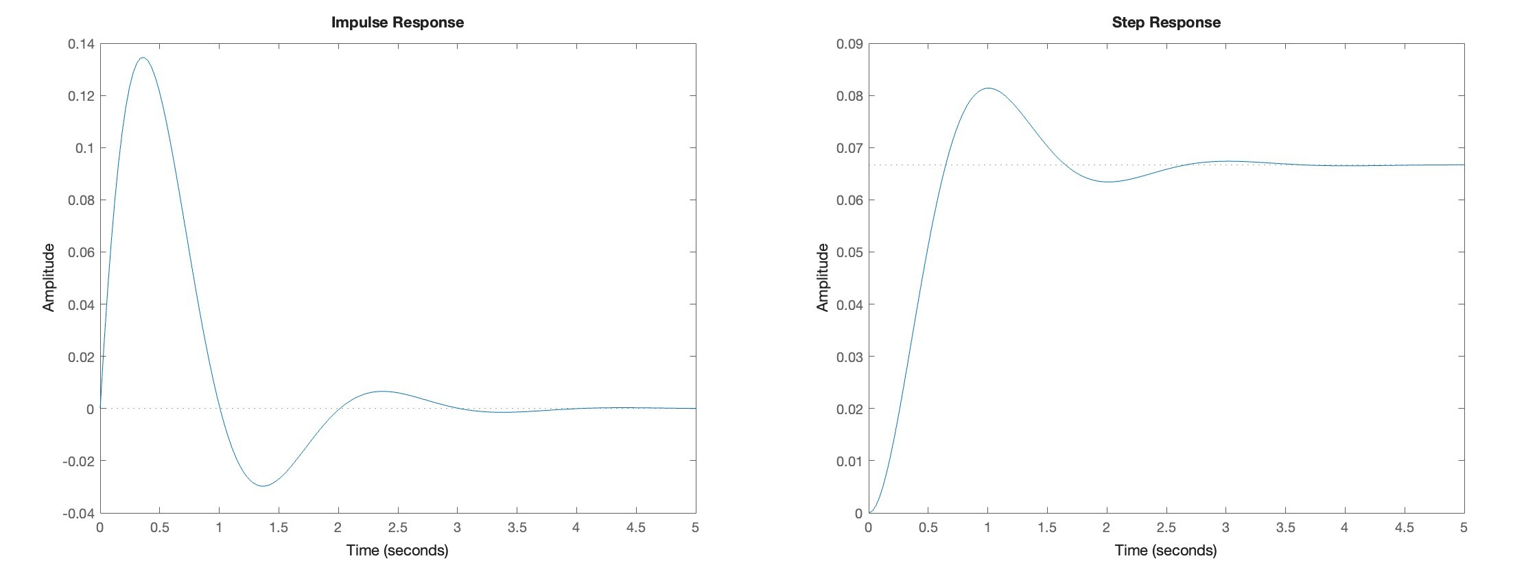
- Harder but more capable way:
num = 0.8;
den = [1 3 12];
sys = tf(num,den);

t = 0:0.1:5;
u = eq(t,0); % delta func
[y,t] = lsim(sys,u,t);
plot(t,y);
grid on;
xlabel('Time');
ylabel('Output');
u = heaviside(t); % unit step func
[y,t] = lsim(sys,u,t);
plot(t,y);
grid on;
xlabel('Time');
ylabel('Output');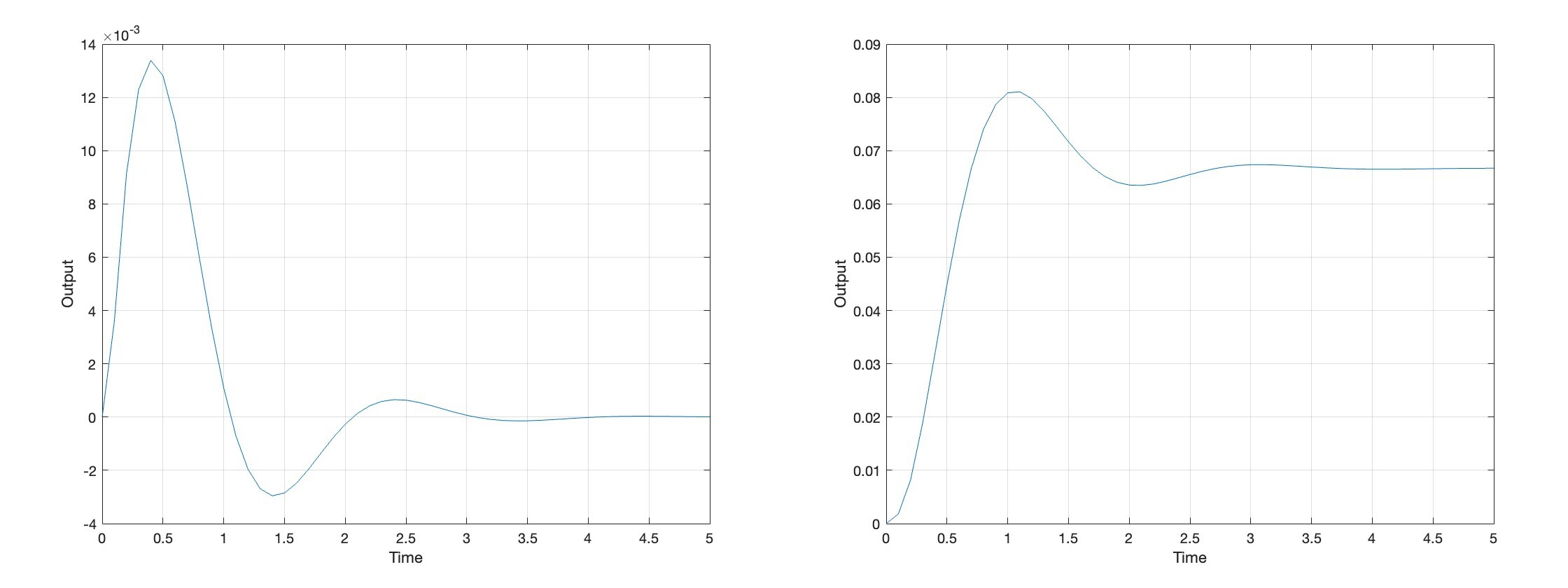
3.2 Student Example 1
Given the RL circuit shown below, use MATLAB to determine the current in the loop and the voltage . Assume , zero initial conditions, and and H.
3.3 Example 2
Implement a state-space representation with lsim(). First, define your system using SSR then the rest of the code is the same as before.
% Define SSR
A = [0 1; -12 -3];
B = [0; 0.8];
C = [1 0];
D = 0;
sys = ss(A,B,C,D);

% Simulate system and plot output
t = 0:0.01:10;
u=heaviside(t);
[y,t] = lsim(sys,u,t);
plot(t,y);
grid on;
xlabel('Time');
ylabel('Output');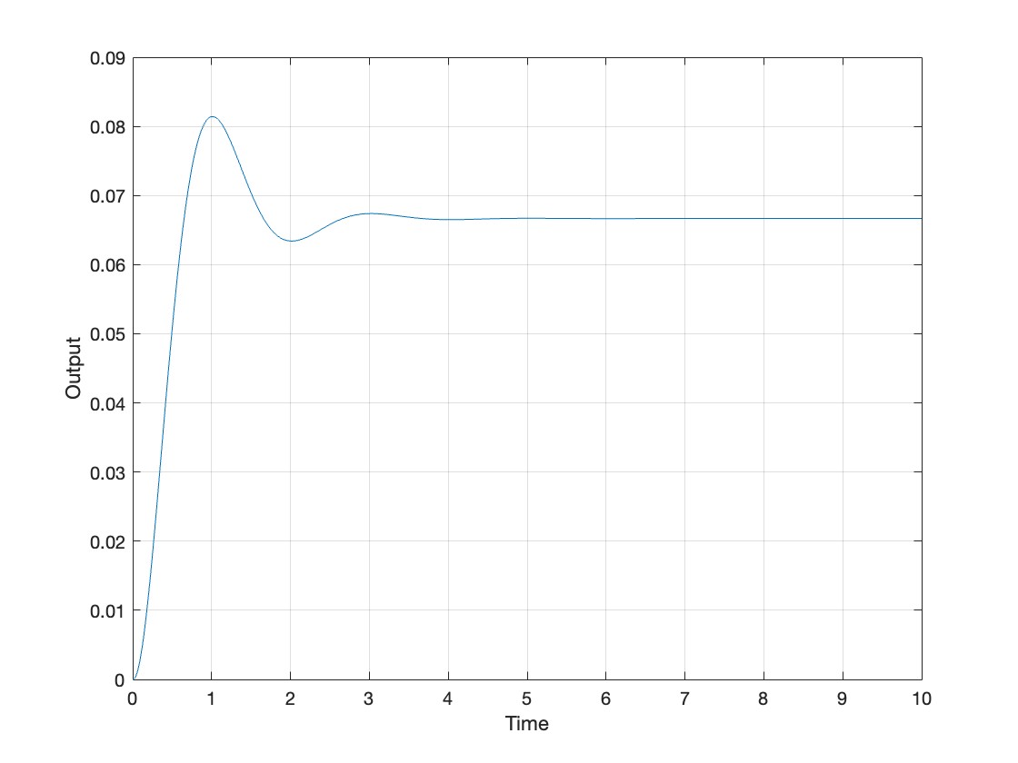
Define initial conditions in state-space like this:
[y,t] = lsim(sys, u, t, x0);Where x0 is the initial state vector (the starting values of each state variable). Just leave x0 off if there are no initial conditions.
4 Simulink - Transfer Functions
Simulink is a graphical way to simulate systems. Behind the scenes, it is numerically solving the differential equations; in other words, it is computing actual values from the equations themselves.
4.1 Example 3
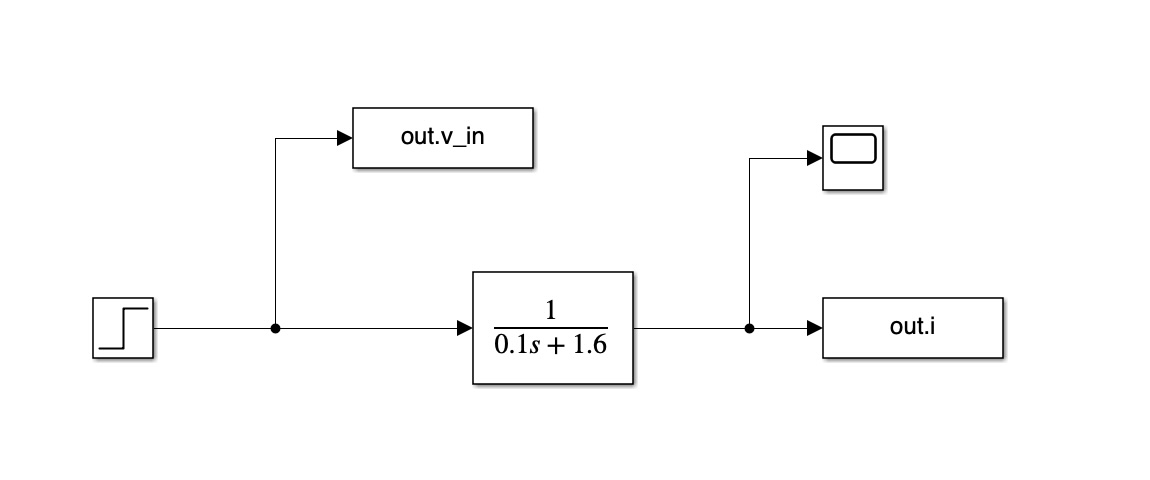
Implement the RL circuit example in Simulink. Plot outputs of the current and . Under Modeling > Model Settings choose ode4 and fixed time step of . For convenience, the transfer function is:
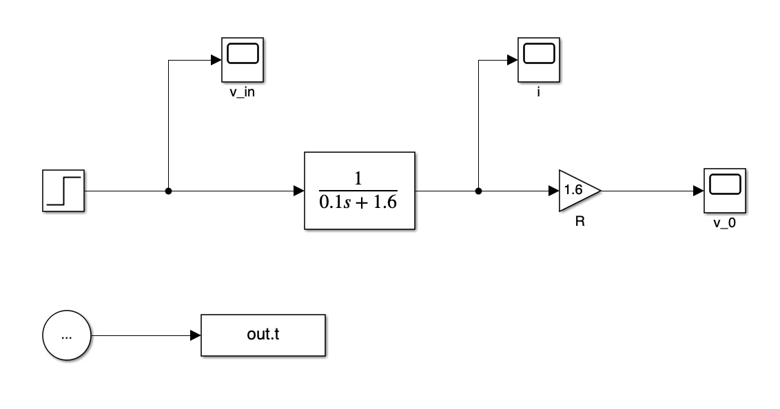
Write output to Workspace if you want to analyze it in MATLAB. Use Scope for output if you want to see the graph. To get the loop current the Simulink would look like this:
To get we have to figure out the voltage across the terminals, which is the current through times .
4.2 Student Example 2
Use Simulink to model the following differential equation of a mechanical system as a transfer function. Assume a step input of magnitude 12 N is applied at sec. Run the simulation to 0.1 sec.
5 Simulink - State Space
State space works essentially the same way as transfer functions. Just choose the State Space box in Simulink instead of the Transfer Function box.
Be sure that the dimensions on your D vector are correct (down x across):
- A matrix:
- B matrix:
- C matrix:
- D matrix:
Define the initial conditions for each state space variable as appropriate.
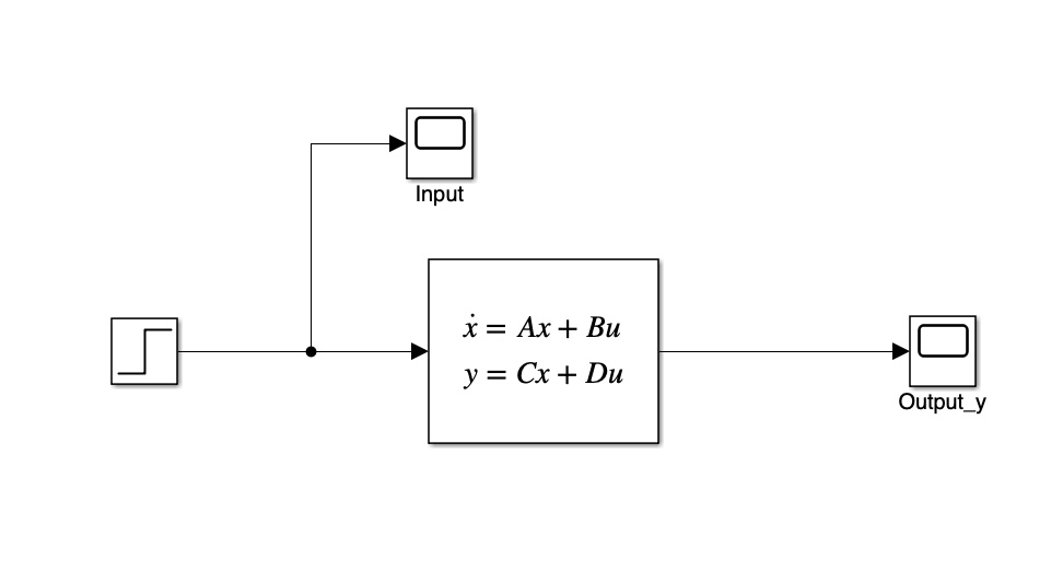
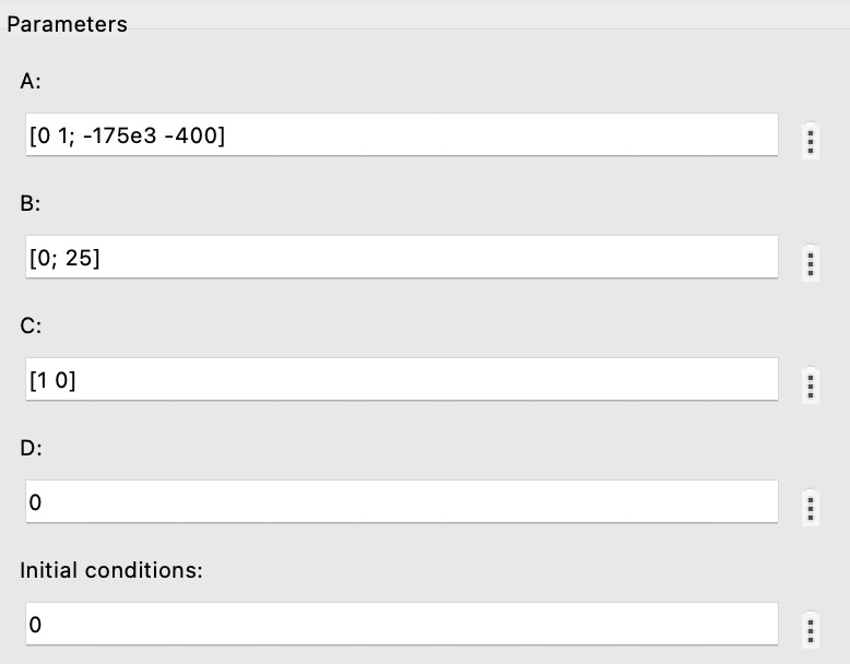
5.1 Example 4
Implement the following state space representation in Simulink. Assume the input is a step input with magnitude 12 N applied at sec. Run the simulation to sec.
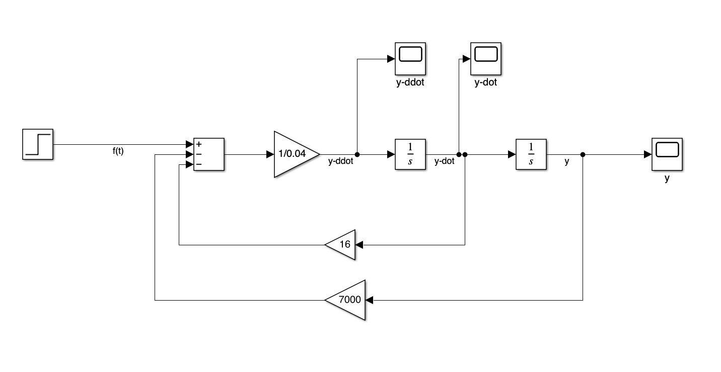
6 Simulink - Integrator Block Method
This method is the easiest to implement because you are basically re-creating the equation using the blocks.
6.1 Example 5
Implement the following DE in Simulink using the integrator block method. Assume a step input applied at sec with a magnitude of 12 N. Run the simulation to sec.