Lesson 21

1 Learning Objectives

By the end of this lesson students will be able to:

Summarize the effect of changing $K_P$ , $K_I$ , and $K_D$ gains on PID controllers
Explain how poles can move without changing system response ( $\zeta$ or $\omega_n$ )

2 Effect of PID Gains on System Response

Recall that a closed-loop system with a PID controller is drawn like this:

TikZ diagram

and has a controller of the form:

$C(s) = K_P + K_D s + \frac{K_I}{s}$

(see Lesson 17). Each gain has a different effect on the system response.

2.1 Proportional Gain, $K_P$

Controller signal proportional to the instantaneous error.
Increase $K_P$ to speed up the system response (reduce peak time $T_P$ ).
Increase $K_P$ to reduce steady-state error.
Increasing $K_P$ increases $\omega_n$ and decreases $\zeta$ (increases overshoot).

2.2 Integral Gain, $K_I$

Control signal proportional to the sum of all past errors. The control signal will be non-zero even if there is no current error.
Increase $K_I$ to reduce steady-state error.
Increasing $K_I$ slows down the system response (increase peak time $T_P$ ).

2.3 Derivative Gain, $K_D$

Control signal proportional to the instantaneous derivative of the error signal.
“Anticipates” the system response because it looks at the rate of change.
Increase $K_D$ to increase $\zeta$ (reduces overshoot and settling time).

2.4 Summary of Gain Effects

The table below summarizes the effect of increasing each gain on the system response:

Gain	Rise Time	Overshoot	Settling Time	SSE
$K_P$	Decrease	Increase	–	Decrease
$K_I$	Increase	Increase	Increase	Eliminate
$K_D$	–	Decrease	Decrease	–

You may not always use $K_P$ , $K_I$ , and $K_D$ depending on the system you are trying to control. For example:

If a system has enough damping, you might set $K_D = 0$ .
If a system has low steady-state error, you might set $K_I = 0$ .

General guidance:

Use $K_P$ to ______________
Use $K_D$ to ______________
Use $K_I$ to ______________

You have three variables that you need to optimize to meet specified response time, overshoot, settling time, and SSE. How do you choose the best values? There are many strategies. We look at one of them today.

2.4.1 Student Exercise 1

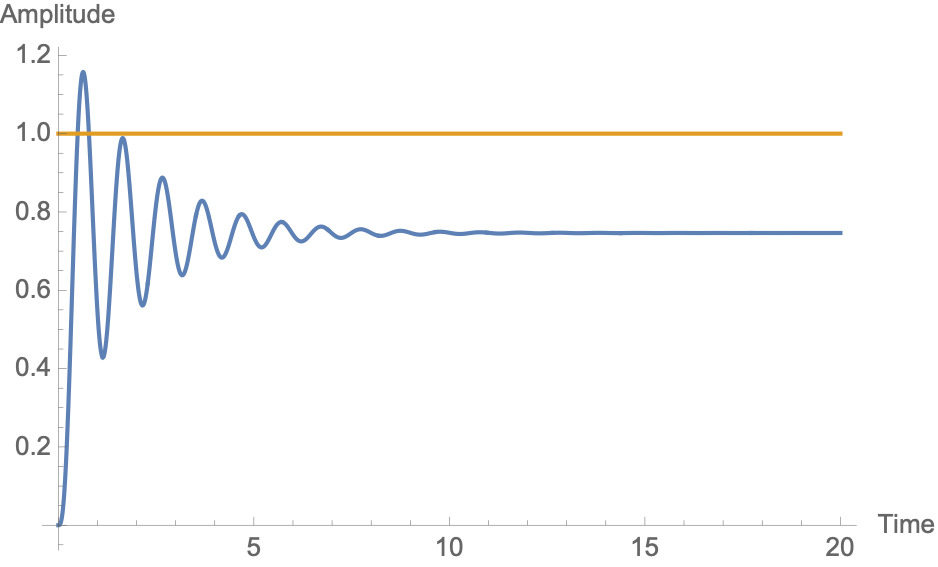
A system produces the step response shown below. You know the system has a PID controller. What gain(s) would you increase or decrease to adjust the system performance to: reduce SSE, decrease rise time, and decrease overshoot?

Figure 1: Step response of a system with a PID controller. The orange line indicates the desired steady-state value.

3 Re-visiting Root Locus Plots

Recall from Lesson 18 that a root-locus plot lets you see the effect of proportional gain on system stability. As $K_P$ increases, the closed-loop poles move along the branches of the plot, and the system response can change from overdamped to underdamped, to marginally stable, to unstable.

When we use a PID controller, things get more complicated. Not only $K_P$ , but also $K_D$ and $K_I$ will move the poles of the system, $T(s)$ .

But we can use root-locus plots for another purpose: designing a specific system response. In a nutshell, $C(s)$ is the way an engineer reliably moves the poles so that the system, $T(s)$ , has the desired performance.

3.1 Pole Location Affects System Performance

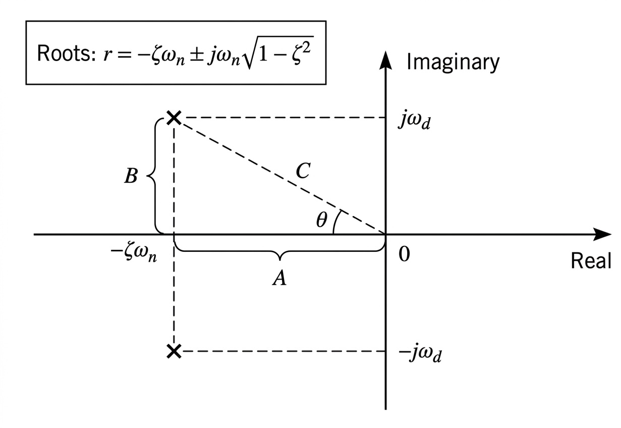
Pole location is determined by the roots of the transfer function denominator. Pole location, in turn, determines system performance. For a second-order system with complex-conjugate poles at $r = -\zeta \omega_n \pm j \omega_n \sqrt{1 - \zeta^2}$ :

$Geometric interpretation of pole location for a second-order system. The real part of the pole sets \zeta \omega_n, the imaginary part sets the damped natural frequency \omega_d, and the angle from the negative real axis sets the damping ratio \zeta.$

Important relationships in the geometric representation:

$\omega_n$ is the hypotenuse of the triangle (i.e., the magnitude of the pole location)
$\zeta = \cos(\theta)$
$\omega_d=\omega_n\sqrt{1-\zeta^2}$

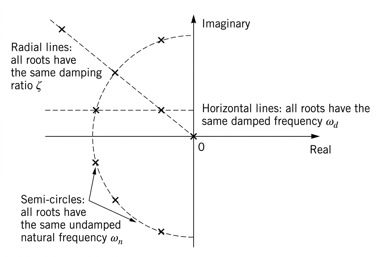
This means that families of pole locations correspond to fixed values of $\zeta$ , $\omega_n$ , and $\omega_d$ :

$Root locations for constant \zeta (radial lines), constant \omega_n (semi-circles), and constant \omega_d (horizontal lines).$

Changing the gain $K_P$ moves the poles along the root-locus plot, which means we can change system performance by changing $K_P$ .

If we adjust $K_P$ we can only adjust system performance to places that exist on the branches of the root locus plot. So if we want the poles in a location off the root-locus plot, we have to change the pole location some other way (i.e., by adding a controller or compensator that introduces new poles or zeros).

Assume we have a unity feedback system with the plant:

$G(s) = \frac{1}{0.5s^2 + 4s + 23}$

And the controller:

$C(s) = K_P + K_D s + \frac{K_I}{s}$

Then $T(s)$ is:

$T(s)=\frac{C(s)G(s)}{1+C(s)G(s)}=\frac{K_D s^2 + K_P s + K_I}{0.5 s^3 + (4 + K_D) s^2 + (23 + K_P) s + K_I}$

So, the three controller constants will impact both pole and zero location. Use the widget below to explore how each affects pole-zero location and the transient response to a unit step input.

But let’s say you want to create a system with specific characteristics. In other words, with a “fast” rise time or a specific natural frequency. Furthermore, what if you wanted to see how your controller settings might affect the system response to a disturbance. For that, you need special tools.