Lesson 9

1 Learning Objectives

By the end of this lesson students will be able to:

• Write the DE for a first order system
• Determine the time constant, rise time, and settling time of a first-order system from its differential equation, sketch, or LaPlace transform, or vice versa
• Sketch the response of a first-order system from its equation or LaPlace transform
• Calculate the steady state value of a first-order system, given its DE or LaPlace transform
• Sketch the response of a first-order system to an impulse or step input

2 Overview

Two methods for observing control system behavior:

1. Time-domain (transient analysis)

• We give the system a mathematically-defined input and calculate what the output looks like
• Shows how the system responds over time (i.e., the transient response)

2. Frequency domain analysis

• Shows how the system output based on the frequency of the input signal
• Shows the steady-state response only

3 Order of the System

The order of the system is the order of the differential equation that describes the system. If multiple DEs are used to describe the system, then the order of the system is the sum of the highest orders from each equation. In this class we cover the transient analysis of first-order and second-order systems.

4 Transient Analysis of a First-Order System DE

The differential equation of a first-order system that is given an input, $F(t)$, and constant coefficients $a$, $b$, and $c$ has the pattern:

$$a\frac{dy}{dt} + by = cF(t)$$

Keep in mind that $y$ changes with time, so it is really $y(t)$, but we are going to just use $y$ to minimize visual clutter.

We are going to re-write the DE above to make it easier to tell how the system will behave. First, we divide through by $b$ and get:

$$\frac{a}{b}\frac{dy}{dt} + y = \frac{c}{b}F(t)$$

Second, we replace $\frac{a}{b}$ with $\tau$ and $\frac{c}{b}$ with $y_{ss}$, the steady-state output of the system:

$$\tau\frac{dy}{dt} + y = y_{ss}F(t)$$

Then, LaPlace transform the equation to get

$$\tau\left( sy(s) - y_{0} \right) + y(s) = y_{ss}F(s)$$

and rearrange to get

$$y(s) = \left( \frac{1}{\tau s + 1} \right)\left( y_{ss}F(s) + \tau y_{0} \right)$$

The solution to this differential equation will depend upon its input. We look at how two inputs, impulse and step, affect the system output $y(t)$.

4.1 Impulse Input

The LaPlace transform for a unit impulse input $F(t) = \delta(t)$ is $F(s) = 1$

$$y(s) = \left( \frac{1}{\tau s + 1} \right)\left( y_{ss}\left( 1 \right) + \tau y_{0} \right)$$

Take the inverse LaPlace transform to get:

$$y(t) = \left( \frac{y_{ss}}{\tau} + y_{0} \right)e^{- \frac{t}{\tau}}$$

4.2 Unit Step Input

The LaPlace transform for a unit step input $F(t) = u(t)$ is $F(s) = \frac{1}{s}$

$$y(s) = \left( \frac{1}{\tau s + 1} \right)\left( y_{ss} \left( \frac{1}{s} \right) + \tau y_{0} \right)$$

Inverse LaPlace to get:

$$y(t) = y_{ss} + \left( y_{0} - y_{ss} \right)e^{- \frac{t}{\tau}}$$

4.3 Initial Conditions

The constant $y_{0}$ is the initial condition of the system. It may be charge in a capacitor, or the initial velocity of a mass. Often, $y_{0} = 0$.

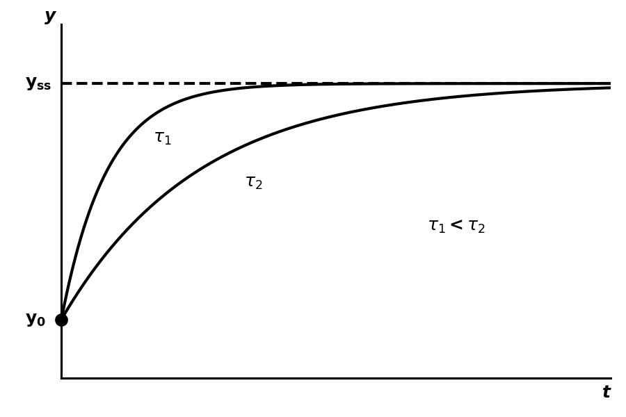
If the system starts out with $y_{0} < y_{ss}$ then the response to a unit step input looks like this:

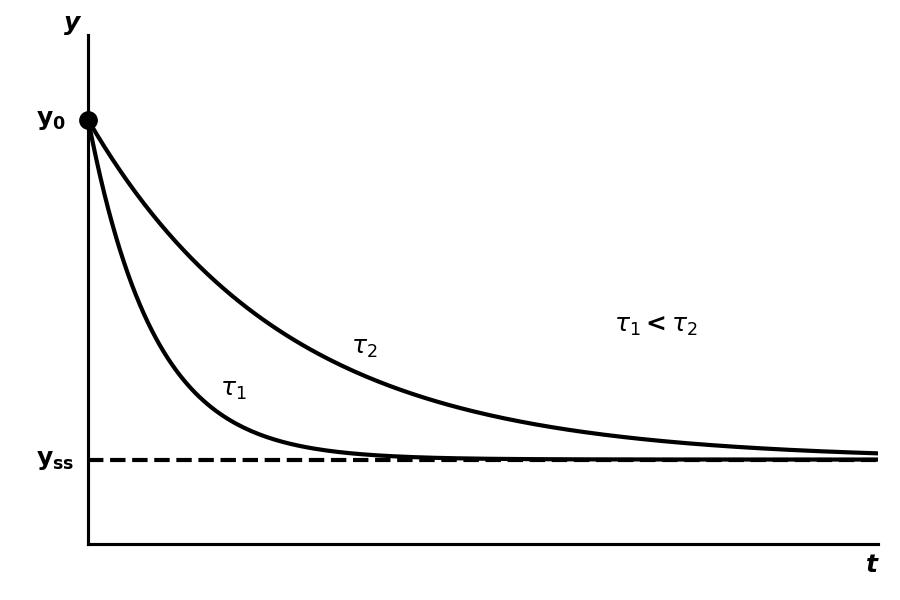
If the system starts out with $y_{0} > y_{ss}$ then the response to a unit step input looks like this:

4.4 Student Example 1

Given: A system modeled by the equation

$$3\frac{dy}{dt} + 14y = 2F(t)$$

and initial condition $y_{0} = 3$

Required: Sketch the transient response to a step input

4.5 Student Example 2

Given: A system modeled by the equation

$$3\frac{dy}{dt} + 2y = 14F(t)$$

and an initial condition $y_{0} = 5$

Required: Sketch the transient response to a step input

5 Key Features of a First-Order System

There are three important features of a system that you should be able to identify from the step response:

1. Time constant, $\tau$
2. Rise time, $T_{r}$
3. Settling time, $T_{s}$

5.1 Time Constant

The time constant is a rule of thumb engineers use to predict how long it takes a system to get to steady state. By convention, one time constant is defined as 63% of the way to the final value. Here’s why:

5.2 Rise Time

The time required for the system output to go from $0.1y_{ss}$ to $0.9y_{ss}$ (10% to 90% of final value). The formula is

$$T_{r} = 2.2\tau$$

5.3 Settling Time

The time required for the system output to reach and stay within 2% of its final value. The formula is

$$T_{s} = 4\tau$$

6 Transient Analysis of a First-Order System by Inspection

Often in controls we do not start with the differential equation. Instead, we start with a block diagram like this:

One of the reasons we use LaPlace notation in controls is because it allows us to determine the time constant and steady-state value by visual inspection.

6.1 Student Example 3

Given: The transfer function below and a step input. Assume $y(0) = 0$.

$$G(s) = \frac{13}{s + 2}$$

Required: (1) Time constant, (2) Steady-state value, (3) Rise time

7 Transient Analysis of a First-Order System with MATLAB

In Lesson 8 we covered two computational ways to get the step response of a system: (1) using the step() function and (2) defining a time range, input function, and running lsim() then plotting the results.

There’s a third approach as well. You can use MATLAB inverse LaPlace transform the equation, analytically solve the equation for $y(t)$, and then plot $y(t)$ over a time range. Use these steps:

1. Write syms s to enable symbolic math in MATLAB.
2. Write y=ilaplace(F(s)*G(s)) and replace F(s) with the LaPlace of your input function and G(s) with the LaPlace of your transfer function.
3. Write fplot(y,[time range]) and replace [time range] with the start and stop times of your plot (e.g., [0 100]).

7.1 Student Example 4

Given: The transfer function below and a step input. Assume $y(0) = 0$.

$$G(s) = \frac{13}{s + 2}$$

Required: Plot the output response in MATLAB in two ways: (1) using tf() and (2) of the solution to the DE using ilplace().

Solution

8 Transient Analysis of a Second-Order System

, and constant coefficients $a$, $b$, and $c$ has the pattern:

The differential equation of a second-order system that is given an input, $F(t)$, and constant coefficients $a$, $b$, $c$, and $d$ has the pattern:

$$a\frac{d^{2}y}{dt^{2}} + b\frac{dy}{dt} + cy = dF(t)$$

Like we did earlier with first-order systems, divide through by $c$ to get

$$\frac{a}{c}\frac{d^{2}y}{dt^{2}} + \frac{b}{c}\frac{dy}{dt} + y = \frac{d}{c}F(t)$$

We create three new substitutions that are unique to second-order systems:

8.1 Natural frequency

$$\omega_{n} = \sqrt{\frac{c}{a}}$$

8.2 Damping ratio

$$\zeta = \frac{b}{2\sqrt{ac}}$$

8.3 Steady-state value

$$y_{ss} = \frac{d}{c}$$

If we use these substitutions, the second-order DE looks like this:

$$\frac{1}{{\omega_{n}}^{2}}\frac{d^{2}y}{dt^{2}} + \frac{2\zeta}{\omega_{n}}\frac{dy}{dt} + y = y_{ss}F(t)$$

If we LaPlace transform, set all initial conditions = 0, and rearrange we get an equation that we can write two different ways.

The first way:

$$y(s) = \left\lbrack \frac{y_{ss}}{\left( \frac{1}{{\omega_{n}}^{2}} \right)s^{2} + \left( \frac{2\zeta}{\omega_{n}} \right)s + 1} \right\rbrack F(s)$$

And the second way:

$$y(s) = \left\lbrack \frac{y_{ss}{\omega_{n}}^{2}}{s^{2} + 2\zeta\omega_{n}s + {\omega_{n}}^{2}} \right\rbrack F(s)$$